REVIEW 4 major objections 6 minor 12 references
Recover Experimental Data with Selection Bias using Counterfactual Logic
T0 review · 4 major / 6 minor · reviewed 2026-08-07 · deepseek-v4-flash
Pith's one-line read A twin-network test decides when selection bias can be undone
desk verdict Theorem 2 is a known adjustment in a new frame, and the continuous simulation's SCM contradicts the randomization assumption, so the empirical claims do not hold as written. read the letter →
The pith
A machine-rendered reading of the paper's core claim, the machinery that carries it, and where it could break.
The reading
What carries the argument
The load-bearing object is the twin network, a graph that pairs each observed variable with a counterfactual copy while sharing the same exogenous noise terms. The paper uses d-separation inside this twin graph as a nonparametric test for whether the selection mechanism reaches the counterfactual outcome. The algebraic work is done by the identity $P(Y^*_{X^*}) = \sum_z P(Y^*_{X^*} \mid Z, S{=}1)\,P(Z)$, which rewrites the unbiased target as a weighted average of biased experimental conditionals, with weights supplied by external population data.
What would settle it
Generate data from a causal model that satisfies the d-separation condition $S \perp\!\!\perp Y^*_{X^*} \mid Z$ in the twin network but in which a hidden common cause of $X$ and $Y$ also influences selection; if the recovered distribution disagrees with the true interventional distribution beyond sampling error, the graphical criterion alone would not be sufficient.
Extended reading notes
Core claim
The paper's central claim is that $P(Y^*_{X^*})$ is s-recoverable from selection-biased experimental data exactly when the twin-network d-separation $S \perp\!\!\perp Y^*_{X^*} \mid Z$ holds for some set $Z$ whose population distribution is known. If $Z$ is empty, the experimental distribution is naturally recoverable: the biased sample already delivers $P(Y^*_{X^*})$. If not, Theorem 2 supplies the weighted-sum identity $P(Y^*_{X^*}) = \sum_z P(Y^*_{X^*} \mid Z, S{=}1)\,P(Z)$. The paper further claims that confounders between $X$ and $Y$ are neither necessary nor sufficient for natural recoverability, and it gives an algorithm that searches over admissible sets $Z$, with a recursive subroutine for cases where an external distribution must itself be recovered.
Load-bearing premise
The recovery formula assumes that, after conditioning on the chosen set $Z$, treatment assignment inside the selected sample is as good as random, so that the observed conditional distribution $P(Y \mid X{=}x, Z, S{=}1)$ equals the counterfactual distribution $P(Y^*_{X^*} \mid Z, S{=}1)$; it also assumes the external population distribution $P(Z)$ is available exactly.
Editorial extensions
If this is right
- If $Y^*_{X^*}$ is d-separated from $S$ by the empty set, the biased experimental dataset already gives the correct experimental distribution, so no external data are needed.
- When the d-separation holds only after conditioning on $Z$, recovery requires exactly the population distribution $P(Z)$; no observational distribution of $Y$ given $X$ is required.
- The algorithm can substitute one admissible external variable set for another, so an unavailable population marginal can sometimes be replaced by a different measurable set.
- Non-recoverability is monotone under edge addition: if a graph cannot be s-recovered, no graph formed by adding edges to it can be s-recovered either.
- Because recovery is decoupled from identification, the method avoids converting $P(Y^*_{X^*})$ into do-calculus form and does not inherit the complications of backdoor identification.
Reading between the lines
- The same twin-network d-separation logic could in principle be applied to other counterfactual queries, such as probabilities of causation, not just the experimental distribution $P(Y^*_{X^*})$.
- If the external distribution $P(Z)$ is only known approximately, the point formula would naturally give way to bounds on the recovered experimental distribution.
- Users should verify that treatment is actually randomized in the selected sample; the paper's own continuous simulation defines $X$ as a function of latent health, which would violate the randomization assumption if taken literally.
- The advanced simulation with selection depending on both $W$ and $Z$ suggests the recovery formula may tolerate more complex selection mechanisms than the simple case, provided the d-separation condition still holds in the twin network.
Editorial analysis
A structured set of objections, weighed in public.
Referee Report
Summary. The paper studies recovery of the experimental/counterfactual distribution P(Y*_X*) from selection-biased experimental data, using twin-network representations of structural causal models. Its main theoretical results are Theorem 1, which states that P(Y*_X*) is naturally recoverable when S and Y*_X* are d-separated by the empty set, and Theorem 2, which gives the recovery formula P(Y*_X*) = sum_z P(Y*_X* | Z, S=1) P(Z) under the conditional independence Y*_X* ⊥ S | Z. The paper also proposes Algorithm 1 for selecting the external adjustment set Z, and it reports discrete and continuous simulation studies claiming to validate the method. The paper frames these results as a complete set of graphical and theoretical criteria for recoverability of experimental distributions under selection bias.
Significance. Theorem 2 is a correct and clean conditioning argument: if the counterfactual outcome is conditionally independent of selection given Z, then external knowledge of P(Z) combined with the biased conditional distribution gives the target distribution. This is a useful observation and it is presented in a way that connects selection-bias recovery to counterfactual/twin-network reasoning rather than to back-door adjustment. The discrete example is internally coherent and illustrates the mechanism. However, the stronger claims in the abstract and introduction—that the paper provides a complete set of criteria and a principled algorithm—are not supported, and the continuous simulation contains a data-generating model that contradicts the estimator's identifying assumption. The theoretical core is defensible, but the paper as written overreaches in several load-bearing places and needs substantial revision.
major comments (4)
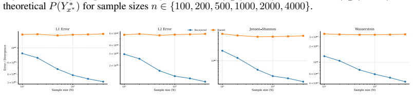
- [§4.2, Table 3] The continuous simulation's SCM contradicts the randomized-assignment assumption on which the estimator relies. Table 3 specifies X = 1{γ_WX W + U_X > 0} with U_X ~ Uniform(0,1), while the text says treatment is 'randomized via a Bernoulli draw.' If γ_WX ≠ 0, then W is a confounder of X and Y, so the KDE estimator of P(Y | X=x, Z, S=1) used in §4.2 is not an estimator of P(Y*_X* | Z, S=1). If γ_WX = 0, the stated formula yields X=1 almost surely, so there is no treatment variation. The results in Table 4 and Figures 4–5 therefore do not validate the recovery procedure under the paper's own data-generating model. The simulation should either specify X ~ Bernoulli(p_X) independently of all other variables or explicitly state and enforce conditional ignorability given the adjustment set actually used.
- [§4.2, paragraph after Table 4] The justification 'since intervening on X does not affect the distribution of S=1 ... P(y*_x* | Z, S=1) = P(y | do(x), Z, S=1)' is incomplete. The fact that S is not caused by X implies P(S=1 | do(x)) = P(S=1), but it does not imply that the observed conditional distribution P(y | X=x, Z, S=1) equals the interventional conditional distribution P(y | do(x), Z, S=1). The latter equality requires a conditional ignorability or randomization assumption, which is exactly what the Table 3 SCM violates. This is a load-bearing gap because the entire estimation step in the continuous experiment depends on this replacement.
- [Algorithm 1 and Lemma 4, §3.2 and Appendix A.4] Algorithm 1 is not a well-defined decision procedure and does not deliver the 'complete set of graphical and theoretical criteria' announced in the abstract. The condition block on lines 6–7 mixes a d-separation test with an assignment statement; line 5 iterates 'foreach set Z∈M' without specifying whether M is a set of variables or a collection of subsets; and the call to RC(Z,∅) is not integrated into a termination or correctness argument. Lemma 4 then concedes that the algorithm does not guarantee a valid output on all graphs. These statements are in tension with the paper's completeness claims. The authors should either prove a completeness theorem for a precisely specified algorithm or substantially weaken the claimed contributions.
- [Lemma 3, Appendix A.2] Lemma 3 is not proven and, as stated, is false. The proof says 'I will only numerically prove the case related to direct paths here, and will provide the proof and analysis based on d-separation later,' but no d-separation argument is ever supplied. Moreover, the lemma claims that natural experimental s-recoverability rules out direct and indirect paths between S and Y, yet Figure 2(a)—which the paper itself classifies as naturally recoverable—contains an indirect path S → X → Y. The lemma needs a precise definition of the paths it covers (for example, paths that do not pass through the intervened node X) or it should be removed, since the central theorems do not rely on it.
minor comments (6)
- [Theorem 1, §3.1] The statement of Theorem 1 uses the condition S ⊥ Y*_X* with no conditioning set, but the proof says 'if X d-separates S from Y*,' which is a different condition. The proof also does not establish the converse direction that would be needed for a 'complete' criterion.
- [Notation, throughout] The paper uses P(Y*_X*), P(Y*_{x*}), and P(y*_x*) with overlapping meaning. These notations should be defined once and used consistently, since the distinction between the counterfactual variable and the value-specific distribution is central to the statements of Theorems 1 and 2.
- [Algorithm 1, §3.2] The pseudocode formatting is broken: the equation P(Y*_x*) = P(Y*_x* | Z, S=1) P(Z) appears inside the if-condition, and the subsequent 'then' and 'return' statements are misaligned. This makes the algorithm hard to parse independently of the text.
- [§4.1 and Appendix A.3.1] In the discrete experiment, the 'true' distribution is computed by back-door adjustment over W even though the treatment is described as randomized. This is not incorrect, but it is unnecessarily indirect and obscures the fact that the recovery formula uses only the external distribution of Z.
- [Language and typos, throughout] There are numerous typographical and grammatical errors, including 'absense,' 'exmaple,' 'experimemtal,' 'Prec(Y*_x*),' and inconsistent capitalization of 'experimental' in the phrase 'natural experimental s-recoverability.' The paper would benefit from careful proofreading.
- [References, §1] Some references are incomplete or malformed, such as 'LaLonde [1986], )' with a stray comma, and the citation style for Bareinboim et al. [2022] is inconsistent with the earlier Bareinboim and Pearl [2012] citation.
Circularity Check
No significant circularity: Theorem 2 is a direct conditioning identity, and the simulations validate rather than define the estimator.
full rationale
The paper's central recovery formula is derived from explicit conditional-independence assumptions rather than from fitted parameters renamed as predictions. Theorem 2 states P(Y*_X*) = sum_z P(Y*_X* | Z, S=1) P(Z) under Y*_X* independent of S given Z, and its proof is a straightforward marginalization plus substitution using that independence; the result is not presupposed in the assumptions, it is the direct algebraic consequence of them. Theorem 1 similarly uses d-separation to certify conditional independence, which is a standard graphical criterion rather than a self-referential definition. The simulation studies generate data from a known SCM and compare the estimator against the same SCM's ground-truth distribution; this is an illustrative validation exercise, not a case where the prediction is forced by the estimator's construction. The paper's references to Pearl, Bareinboim, and others are external foundational works, and no load-bearing argument reduces to a self-citation. The continuous-experiment SCM's equation for X in Table 3 may conflict with the stated Bernoulli randomization assumption, but that is a correctness and validity concern, not a circularity concern.
Assumptions & free parameters
assumptions (5)
- standard math Twin network with shared exogenous variables correctly represents counterfactual quantities and conditional independences.
- standard math P(Y*_X*) equals the interventional distribution P(y|do(x)).
- domain assumption The experimental sample is generated with treatment randomization, so P(Y*_X*|Z,S=1) can be estimated from observed P(Y|X=x,Z,S=1).
- domain assumption The external unbiased distribution P(Z) is available and equals the target population distribution.
- standard math d-separation is sound and complete for the compatible distributions, including faithfulness.
Cite this review
Pith. "Pith review of Recover Experimental Data with Selection Bias using Counterfactual Logic." pith.science (2026). https://pith.science/paper/FBU7PM36
@misc{pith2026250600335,
  author       = {Pith},
  title        = {Pith review of: Recover Experimental Data with Selection Bias using Counterfactual Logic},
  year         = {2026},
  howpublished = {\url{https://pith.science/paper/FBU7PM36}},
  note         = {Machine review of arXiv:2506.00335}
}
abstract
Selection bias, arising from the systematic inclusion or exclusion of certain samples, poses a significant challenge to the validity of causal inference. While Bareinboim et al. introduced methods for recovering unbiased observational and interventional distributions from biased data using partial external information, the complexity of the backdoor adjustment and the method's strong reliance on observational data limit its applicability in many practical settings. In this paper, we formally discover the recoverability of $P(Y^*_{x^*})$ under selection bias with experimental data. By explicitly constructing counterfactual worlds via Structural Causal Models (SCMs), we analyze how selection mechanisms in the observational world propagate to the counterfactual domain. We derive a complete set of graphical and theoretical criteria to determine that the experimental distribution remain unaffected by selection bias. Furthermore, we propose principled methods for leveraging partially unbiased observational data to recover $P(Y^*_{x^*})$ from biased experimental datasets. Simulation studies replicating realistic research scenarios demonstrate the practical utility of our approach, offering concrete guidance for mitigating selection bias in applied causal inference.
Figures


Figures from the paper (8 more)



Reference graph
Works this paper leans on
- [1]
-
[2]
if and only ifZblocks every path from a node inXto a node inYand is denoted byY⊥ ⊥X|Z
Every other node on the path is outsideZ. if and only ifZblocks every path from a node inXto a node inYand is denoted byY⊥ ⊥X|Z. Theorem 3(Soundness & Completeness of d -separation (Pearl [2014], Geiger et al. [1990], Verma and Pearl [2022])).Let G be a DAG and P a joint distribution over its nodes. If P satisfies the global Markov property w.r.t. G and t...
work page 2014
-
[3]
Remove all incoming edges into each node inXto obtain the mutilated graphG do(X)
-
[4]
Fix eachX∈Xto the valuex, while all other variables remain governed by their original structural equations. The resulting interventional (or experimental) distribution is P Y|do(X=x),Z=z =P Gdo(X) Y|Z=z,X=x , which generally differs from the observational conditionalP(Y|X=x,Z=z). Definition 5(Counterfactuals Pearl et al. [2000]).Given a structural causal ...
work page 2000
-
[5]
Identify the unique exogenous assignmentusatisfying the evidencee
-
[6]
Modify the model M by replacing the structural equations of each X∈X with the constant x′, yielding the mutilated modelM x′
-
[7]
the ultimate level of causal hierarchy
Evaluate the sentence Y(u) =y inM x′. Pearl defines this as “the ultimate level of causal hierarchy” and denotes such queries as P Yx′ =y|e . Definition 6(s-recoverability(Bareinboim et al. [2022])).Given a causal graph Gs augmented with a node S encoding the selection mechanism Bareinboim and Pearl [2012], the distribution Q=P(y|x) is said to bes-recover...
work page 2022
-
[8]
IfW∪Z⊆T, thenP(W|Z)is s-recoverable
Show all 12 references
-
[9]
If S⊥ ⊥W Z, thenP(W|Z)is s-recoverable as P(W|Z) =P(W|Z, S= 1)
-
[10]
IfC∪Z⊆T, thenP(W|Z)is s-recoverable
For minimalC⊆Msuch thatS⊥ ⊥W Z∪C, P(W|Z) = X c P(W|Z, c, S= 1)P(c|Z). IfC∪Z⊆T, thenP(W|Z)is s-recoverable. Otherwise, callRC(C, Z)
-
[11]
CallRC W ′,{W\W ′} ∪Z andRC W\W ′, Z
For someW ′ ⊂W, P(W|Z) =P W ′|W\W ′, Z P W\W ′|Z . CallRC W ′,{W\W ′} ∪Z andRC W\W ′, Z
-
[12]
A.2 Lemmas and Proofs X Y S W M M ∗ W ∗ S∗ X ∗ Y ∗ UM US UW UY UX Figure 6: There are direct path, indirect path, and spurious path betweenYandS
Exit withFAIL(to s-recover P(W|Z) ) if for a singleton W , none of the above operations are applicable. A.2 Lemmas and Proofs X Y S W M M ∗ W ∗ S∗ X ∗ Y ∗ UM US UW UY UX Figure 6: There are direct path, indirect path, and spurious path betweenYandS. Lemma 2.If experimental dis...
2000
Reviewed August 7, 2026 · model on record in the stance chip above.
Discussion (0). Sign in to comment.