REVIEW 3 major objections 5 minor 57 references
Real-time Light Curve Classification Framework for the Wide Field Survey Telescope Using Modified Semi-supervised Variational Auto-Encoder
T0 review · 3 major / 5 minor · reviewed 2026-08-07 · deepseek-v4-flash
Pith's one-line read This paper claims that adding an unsupervised reconstruction path to a supervised classifier improves early transient classification: on simulated WFST data it reaches 83.1% accuracy at three days after trigger, versus 78.7% for an RNN…
desk verdict Useful early-classification framework for WFST simulations, but the claimed 5.59% semi-supervised gain is not actually demonstrated and needs an ablation before I'd trust it. read the letter →
The pith
A machine-rendered reading of the paper's core claim, the machinery that carries it, and where it could break.
The reading
What carries the argument
The load-bearing object is a semi-supervised variational auto-encoder with one shared encoder and two branches. The supervised branch maps the latent code to class probabilities through a softmax layer; the unsupervised branch decodes the latent code into the full 90-day light curve. The input is the three-day partial light curve in the u, g, and r bands, with later time steps masked to zero, and the reconstruction target is the full light curve. These branches are trained together with a total loss $\mathcal{L}_{\mathrm{tot}} = W_r \mathcal{L}_{\mathrm{rec}} + W_k \mathcal{L}_{\mathrm{KL}} + W_c \mathcal{L}_{\mathrm{cla}}$, where $\mathcal{L}_{\mathrm{rec}}$ is reconstruction mean squared error, $\mathcal{L}_{\mathrm{KL}}$ is the Kullback-Leibler divergence to a Gaussian prior, and $\mathcal{L}_{\mathrm{cla}}$ is categorical cross-entropy, with $W_c = 10$ so that the classification term dominates. The variational formulation keeps the latent space continuous and structured, so neighboring latent points decode to similar light curves.
What would settle it
Train both the framework and the RNN benchmark on the same simulated sample, then apply them to a set of spectroscopically confirmed transients from WFST's real alert stream, classifying each at three days after trigger with identical preprocessing. If the framework's accuracy does not exceed the benchmark's by a comparable margin, or falls below it, the central claim that the reconstruction path improves early classification in practice is falsified.
Extended reading notes
Core claim
On simulated WFST-like light curves drawn from PLAsTiCC models via SNANA, the paper finds that coupling a supervised classification branch with an unsupervised variational auto-encoder that reconstructs the full light curve from the partial early light curve improves early classification. Across 10-fold cross-validation, the framework reaches 83.1 percent accuracy at three days after trigger, compared with 78.7 percent for a GRU-based RNN benchmark, and raises macro precision and recall from 0.836 to 0.858. The authors attribute the gain to the reconstruction task: the shared encoder must encode enough information about the full evolution to reconstruct it, so the early-phase representation carries more class-discriminative content than a purely supervised RNN would learn. They also show that the latent space clusters by class and that reconstruction of the full curve is possible, with an average reconstruction loss of 19.56 percent.
Load-bearing premise
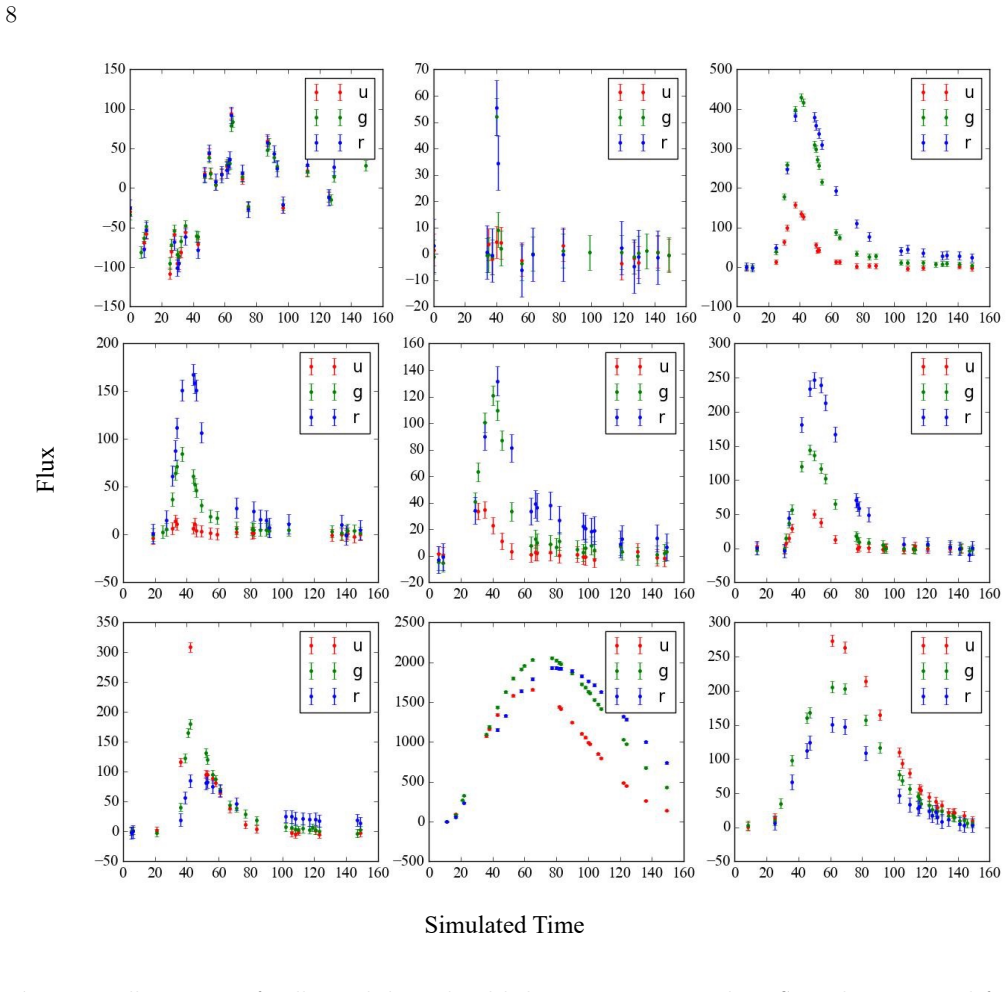
The load-bearing premise is that the simulated light curves—generated from PLAsTiCC models with the SNANA package, smoothed by Gaussian processes, and split by redshift—are representative enough of real WFST observations that the measured 5.59 percent accuracy gain will transfer to the alert stream.
Editorial extensions
If this is right
- At three days after trigger, the framework separates nine transient classes at 83.1 percent accuracy on simulated data, making early follow-up of fast-evolving events such as kilonovae and tidal disruption events feasible.
- Because the encoder is shared, every classified alert also carries a reconstructed full light curve and a latent code; the paper identifies anomaly detection and observation-phase determination as downstream uses.
- The framework can be updated with newly collected unlabeled data without discarding previously learned structure, which the paper argues matters for a new survey whose labeled sample is small.
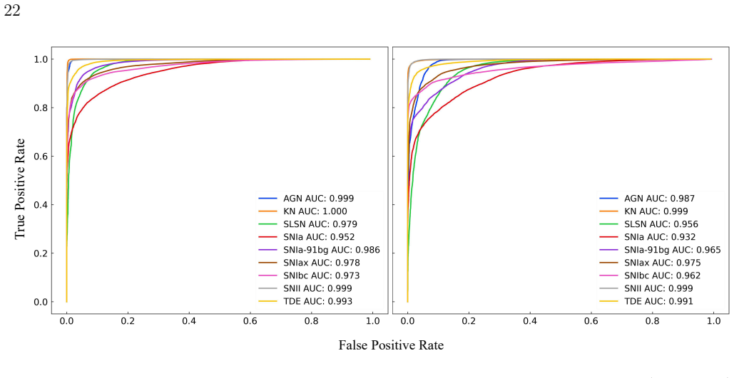
- Precision and recall improve in almost all subclasses relative to the GRU benchmark, with the largest absolute gains in classes such as AGN and TDE.
- The performance advantage over the benchmark appears from the early phase onward and remains consistent as more data accumulate, according to the paper's phase-resolved comparison.
Reading between the lines
- A natural test the paper does not run is to vary the amount of unlabeled data and the label fraction; the hypothesis that reconstruction helps most when labels are scarce is directly measurable and would tell observers how much spectroscopic follow-up is needed.
- Because the reconstruction target is the full light curve, the same architecture can be read as a forecasting device: at three days it predicts the upcoming 87 days, so its output could seed trigger decisions for time-critical follow-up even before the classifier's probability is used.
- The paper's own latent-space plot of the unseen CART class suggests a practical anomaly detector: alerts that land far from known clusters, or that reconstruct poorly, could be prioritized for human review even if the classifier assigns them a known label.
- The relative comparison between the two models on identical simulated input is probably a safer quantity to carry into the real survey than the absolute 83.1 percent accuracy, since simulation bias affects both models similarly; the paper makes this point only implicitly.
Editorial analysis
A structured set of objections, weighed in public.
Referee Report
Summary. The paper presents a semi-supervised variational auto-encoder (VAE) framework for early classification of simulated Wide Field Survey Telescope (WFST) light curves. The framework combines a supervised GRU-based classification path with an unsupervised decoder path that reconstructs a full 90-day light curve from a partial input covering only the first three days after trigger. Evaluated on SNANA-generated, PLAsTiCC-based simulated light curves, the authors report an accuracy of 0.831 versus 0.787 for a GRU benchmark model, with improvements in precision and recall for most subclasses. The paper also presents latent-space visualizations and light-curve reconstructions, and states that the code and model weights are publicly available. The core claim is that the unsupervised reconstruction path and the use of unlabeled data drive the observed accuracy improvement.
Significance. If the reported improvement is real and can be causally attributed to the proposed semi-supervised reconstruction mechanism, the framework would be a practically useful contribution to early transient classification, where rapid follow-up decisions matter. The paper addresses a relevant problem, uses a realistic simulation pipeline (SNANA with PLAsTiCC models and WFST cadence), makes code and model weights available, and explicitly acknowledges the limitations of simulated data for real-world transfer. However, the central causal claim—that the unsupervised path is responsible for the accuracy gain—is not established by the experiments as presented, because the comparison against the benchmark is confounded by multiple simultaneous differences and no ablation studies are reported. The significance of the work therefore hinges on additional controlled experiments that isolate the contribution of each component.
major comments (3)
- [Section 4.4, Table 4, Eq. (6)] The headline improvement (accuracy 0.831 vs 0.787) is attributed to the unsupervised auto-encoder path, but the comparison does not isolate this mechanism. The full framework differs from the GRU benchmark in at least three ways: the decoder branch and reconstruction loss L_rec (Eq. 3), the KL loss L_KL (Eq. 4), and the inclusion of an additional unlabeled training dataset. No experiments vary the loss weights W_r, W_k, W_c in Eq. (6) or the amount/composition of the unlabeled data, and no parameter counts or training budgets are reported for the two models. As a result, the measured gain could be due to added model capacity, multi-task regularization from the reconstruction branch, or simply seeing more training examples, rather than the claimed semi-supervised representation learning. Please add ablations: (a) the supervised path trained alone (no decoder or KL terms), (b) the full framework trained with labeled data only, and (c) the full framework trained with varying amounts of unlabeled data, to demonstrate the specific contribution of each component.
- [Section 4, first paragraph] The evaluation protocol is described as "10-fold cross-validation (each fold contains approximately 2000 light curves, randomly selected from the test dataset without specific division)". This is not the standard use of cross-validation, which is typically performed on the training set for model selection, with the test set held out for final evaluation. As written, it is unclear whether the reported accuracy and uncertainties come from training on the test set, from repeated random subsampling of the test set, or from some other procedure. This ambiguity directly affects the validity of the reported accuracy uncertainty (0.012) and the fairness of the comparison with the benchmark model. Please clarify the exact protocol: how many models were trained, how the folds were created, whether the same folds were used for both models, and whether any training data were used in the cross-validation procedure.
- [Section 3.3.2, Eq. (5)] The framework is described as semi-supervised, and Section 4.4 implies that the use of unlabeled data contributes to the accuracy gain, but the loss function L_cla (Eq. 5) is defined only for labeled samples, and the text does not specify how unlabeled samples enter the training objective. If unlabeled samples contribute only through L_rec and L_KL, then the claimed benefit of unlabeled data is not independent of the reconstruction regularization, and the term "semi-supervised" is potentially misleading. Please state explicitly whether unlabeled samples enter L_cla (e.g., via pseudo-labels or a weighted cross-entropy term) and, if they do not, revise the claims about the role of unlabeled data accordingly.
minor comments (5)
- [Section 3.3.2] In the paragraph after Eq. (6), the text says the overall loss is "combined as outlined in Equation 5", but the total loss is defined in Eq. (6); the equation number should be corrected.
- [Section 4.2] The passage "we exclude the CART (Calcium-rich gap transients) class in the training dataset" is confusing because CART is not listed among the nine classes in Table 1 or in the dataset description in Section 2.2; please clarify whether CART was part of the simulated data and, if so, why it is excluded, or remove this passage if it is an error.
- [Tables 2 and 3] The reported uncertainties are given to three significant figures (e.g., 4.8E-04), which seems overly precise given that the standard deviation across folds is not described; consider reporting fewer significant digits or explaining explicitly how these uncertainties were computed from the evaluation procedure.
- [Section 3.3.1] The phrase "masking the values after a certain time step with zeros" is ambiguous: are zeros used as input features alongside a masking layer in the GRU, or is the zero-padding itself the only indicator? The architecture in Figure 5 includes a masking operation, but the text should specify that zeros are used with a mask to distinguish unobserved time steps.
- [Abstract / Code availability] The abstract and GitHub mention state that code and model weights are publicly available, but no repository URL or data availability statement is provided in the manuscript; adding the URL would help reproducibility.
Circularity Check
No circularity: the headline accuracy gain is an empirical comparison on a held-out simulated test set, and the reconstruction path is a trained objective, not an independent prediction; the missing ablation is an attribution concern, not circularity.
full rationale
The paper's central claim is an empirical model comparison: the full semi-supervised framework reaches accuracy 0.831 versus 0.787 for a benchmark RNN on the same simulated test set, evaluated by 10-fold cross-validation. This is not a derivation from assumptions, and the test set is held out from training, so the comparison is not circular by construction. The reconstruction path is trained with the explicit mean-square-error objective in Eq. 3 to map a partial light curve to the full light curve; reporting a test reconstruction loss of 19.56% is a standard evaluation of that same objective, not a claim that the reconstruction is an independent, untrained prediction. The paper does not invoke a uniqueness theorem, does not define any central quantity in terms of another claimed result, and does not rely on a load-bearing self-citation chain; the only co-authored citation (Cai et al. 2025, which includes author L. Fan) concerns the WFST alert stream and is not used to justify the classification improvement. The absence of an ablation isolating the unsupervised path means the causal attribution in Section 4.4 is underdetermined, but that is a correctness/interpretability limitation, not circularity, because the headline gain is still a direct measurement on a separate test set rather than a quantity that reduces to a fitted input or to a self-citation. The paper's own limitation note that simulated-data performance may be overly optimistic concerns external validity, not circular derivation. Therefore no circular step can be exhibited, and the score is 0.
Assumptions & free parameters
free parameters (8)
- Loss weights Wr, Wk, Wc =
Wr=1, Wk=1, Wc=10
- Network architecture hyperparameters (layers, units) =
Not given numerically in text; topology shown in Figures 6-7
- Latent dimensionality =
2 (implied by latent space plots)
- GP kernel hyperparameters =
Matern-3/2 length scales, fitted per light curve
- Early classification window =
3 days after trigger (phase j=6)
- Global normalization constant F =
Maximum flux across all training data
- Trigger threshold =
5-sigma in imaging difference
- GP augmentation wavelength shifts =
Described as low/high 'z' scenarios; exact shift values not given
assumptions (6)
- domain assumption PLAsTiCC simulation models faithfully represent the nine transient classes and their light-curve properties.
- domain assumption SNANA with custom SIMLIB and survey definition reproduces WFST cadence, filters, and depth.
- domain assumption GP interpolation with a Matern-3/2 kernel provides unbiased 90-day light curves from sparse early data.
- ad hoc to paper The reconstruction target, the GP-interpolated full light curve, is the correct learning target for the unsupervised path.
- ad hoc to paper Zero-padding unobserved future time steps, without feeding the phase index to the network, is sufficient for the model to know how much of the curve is observed.
- domain assumption Train and test sets with identical class distributions, split only by redshift, are adequate for evaluating generalization.
Cite this review
Pith. "Pith review of Real-time Light Curve Classification Framework for the Wide Field Survey Telescope Using Modified Semi-supervised Variational Auto-Encoder." pith.science (2026). https://pith.science/paper/7AVXELBM
@misc{pith2026250601216,
  author       = {Pith},
  title        = {Pith review of: Real-time Light Curve Classification Framework for the Wide Field Survey Telescope Using Modified Semi-supervised Variational Auto-Encoder},
  year         = {2026},
  howpublished = {\url{https://pith.science/paper/7AVXELBM}},
  note         = {Machine review of arXiv:2506.01216}
}
read the original abstract
Modern time-domain astronomy will benefit from the vast data collected by survey telescopes. The 2.5 m Wide Field Survey Telescope (WFST), with its powerful capabilities, is promising to make significant contributions in the era of large sky surveys. To harness the full potential of the enormous amount of unlabeled light curve data that the WFST will collect, we have developed a semisupervised light curve classification framework. This framework showcases several unique features. First, it is optimized for classifying events based on the early phase of the light curve (three days after trigger), which can help identify interesting events early and enable efficient follow-up observations. Second, the semisupervised nature of our framework allows it to leverage valuable information from large volumes of unlabeled data, potentially bridging the gap between simulations and real observations and achieving better generalization in practical scenarios. Compared to the commonly used Recurrent Neural Network models, our framework has shown a 5.59% improvement in accuracy for early classification tasks, as well as improvements in precision and recall in almost all subclasses. Moreover, our approach provides a reconstructed light curve, along with a compact latent representation, offering a different perspective that can be used for further downstream tasks beyond classification. The code and model weights used in this work are maintained and publicly available on our GitHub repository.
Figures


Figures from the paper (10 more)




Reference graph
Works this paper leans on
-
[1]
2024, PASP, 136, 124504, doi: 10.1088/1538-3873/ad9a7d
Abdelhadi, B., & Rubin, D. 2024, PASP, 136, 124504, doi: 10.1088/1538-3873/ad9a7d
-
[2]
2019, MNRAS, 482, 5078, doi: 10.1093/mnras/sty2836
Aguirre, C., Pichara, K., & Becker, I. 2019, MNRAS, 482, 5078, doi: 10.1093/mnras/sty2836
-
[3]
Allam, T., & McEwen, J. D. 2024, RAS Techniques and Instruments, 3, 209, doi: 10.1093/rasti/rzad046
-
[4]
Allam, Jr., T., Peloton, J., & McEwen, J. D. 2023, arXiv e-prints, arXiv:2303.08951, doi: 10.48550/arXiv.2303.08951
work page Pith review arXiv doi:10.48550/arxiv.2303.08951 2023
-
[5]
Greengard, L., Hogg, D. W., & O’Neil, M. 2015, IEEE Transactions on Pattern Analysis and Machine Intelligence, 38, 252, doi: 10.1109/TPAMI.2015.2448083
arXiv 2015
-
[6]
2019, arXiv e-prints, arXiv:1904.07248, doi: 10.48550/arXiv.1904.07248
Baron, D. 2019, arXiv e-prints, arXiv:1904.07248, doi: 10.48550/arXiv.1904.07248
-
[7]
2020, MNRAS, 493, 2981, doi: 10.1093/mnras/staa350
Becker, I., Pichara, K., Catelan, M., et al. 2020, MNRAS, 493, 2981, doi: 10.1093/mnras/staa350
-
[8]
Bellm, E. C., Kulkarni, S. R., Graham, M. J., et al. 2019, PASP, 131, 018002, doi: 10.1088/1538-3873/aaecbe
Show all 57 references
-
[9]
A., Abe, F., Dodd, R
Bond, I. A., Abe, F., Dodd, R. J., et al. 2001, MNRAS, 327, 868, doi: 10.1046/j.1365-8711.2001.04776.x
2001
-
[10]
2019, AJ, 158, 257, doi: 10.3847/1538-3881/ab5182 —
Boone, K. 2019, AJ, 158, 257, doi: 10.3847/1538-3881/ab5182 —. 2021, AJ, 162, 275, doi: 10.3847/1538-3881/ac2a2d 29
2019 doi
-
[11]
F., & Maund, J
Burhanudin, U. F., & Maund, J. R. 2023, MNRAS, 521, 1601, doi: 10.1093/mnras/stac3672
2023 doi
-
[12]
2025, arXiv e-prints, arXiv:2501.15018, doi: 10.48550/arXiv.2501.15018
Cai, M., Xu, Z., Fan, L., et al. 2025, arXiv e-prints, arXiv:2501.15018, doi: 10.48550/arXiv.2501.15018
2025 doi
- [13]
- [14]
-
[15]
2015, Keras, https://keras.io Dark Energy Survey Collaboration, Abbott, T.,
Chollet, F., et al. 2015, Keras, https://keras.io Dark Energy Survey Collaboration, Abbott, T.,
2015
- [16]
-
[17]
2023, A&A, 670, A54, doi: 10.1051/0004-6361/202243928
Donoso-Oliva, C., Becker, I., Protopapas, P., et al. 2023, A&A, 670, A54, doi: 10.1051/0004-6361/202243928
2023 doi
-
[18]
J., Djorgovski, S
Drake, A. J., Djorgovski, S. G., Mahabal, A., et al. 2012, in IAU Symposium, Vol. 285, New Horizons in Time Domain Astronomy, ed. E. Griffin, R. Hanisch, & R. Seaman, 306–308, doi: 10.1017/S1743921312000889
2012 doi
-
[19]
2017, A&A, 603, A60, doi: 10.1051/0004-6361/201630240
Frontera-Pons, J., Sureau, F., Bobin, J., & Le Floc’h, E. 2017, A&A, 603, A60, doi: 10.1051/0004-6361/201630240
2017 doi
-
[20]
I., & Aleo, P
Malz, A. I., & Aleo, P. D. 2023, ApJ, 954, 6, doi: 10.3847/1538-4357/ace326 Hloˇ zek, R., Malz, A. I., Ponder, K. A., et al. 2023, ApJS, 267, 25, doi: 10.3847/1538-4365/accd6a
2023 doi
-
[21]
1997, Neural computation, 9, 1735
Hochreiter, S., & Schmidhuber, J. 1997, Neural computation, 9, 1735
1997
-
[22]
2020, MNRAS, 493, 6050, doi: 10.1093/mnras/staa642
Hosenie, Z., Lyon, R., Stappers, B., Mootoovaloo, A., & McBride, V. 2020, MNRAS, 493, 6050, doi: 10.1093/mnras/staa642
2020 doi
-
[23]
2022a, ApJ, 936, 157, doi: 10.3847/1538-4357/ac7394
Hu, L., Wang, L., Chen, X., & Yang, J. 2022a, ApJ, 936, 157, doi: 10.3847/1538-4357/ac7394
-
[24]
2022b, Universe, 9, 7, doi: 10.3390/universe9010007 Ivezi´ c,ˇZ., Kahn, S
Hu, M., Hu, L., Jiang, J.-a., et al. 2022b, Universe, 9, 7, doi: 10.3390/universe9010007 Ivezi´ c,ˇZ., Kahn, S. M., Tyson, J. A., et al. 2019, ApJ, 873, 111, doi: 10.3847/1538-4357/ab042c
2019 doi
-
[25]
Jamal, S., & Bloom, J. S. 2020, ApJS, 250, 30, doi: 10.3847/1538-4365/aba8ff
2020 doi
-
[26]
2012, in AAS/Division for Planetary Sciences Meeting
Jedicke, R., Tonry, J., Veres, P., et al. 2012, in AAS/Division for Planetary Sciences Meeting
2012
-
[27]
2010, in Society of Photo-Optical Instrumentation Engineers (SPIE) Conference
Kaiser, N., Burgett, W., Chambers, K., et al. 2010, in Society of Photo-Optical Instrumentation Engineers (SPIE) Conference
2010
-
[28]
7733, Ground-based and Airborne Telescopes III, ed
Series, Vol. 7733, Ground-based and Airborne Telescopes III, ed. L. M. Stepp, R. Gilmozzi, & H. J. Hall, 77330E, doi: 10.1117/12.859188
-
[29]
P., Cinabro, D., et al
Kessler, R., Bernstein, J. P., Cinabro, D., et al. 2009, PASP, 121, 1028, doi: 10.1086/605984
2009 doi
-
[30]
2019, PASP, 131, 094501, doi: 10.1088/1538-3873/ab26f1
Kessler, R., Narayan, G., Avelino, A., et al. 2019, PASP, 131, 094501, doi: 10.1088/1538-3873/ab26f1
2019 doi
-
[31]
2023, Research in Astronomy and Astrophysics, 23, 035013, doi: 10.1088/1674-4527/acb877 30
Lei, L., Zhu, Q.-F., Kong, X., et al. 2023, Research in Astronomy and Astrophysics, 23, 035013, doi: 10.1088/1674-4527/acb877 30
2023 doi
-
[32]
2022, MNRAS, 513, 2422, doi: 10.1093/mnras/stac946
Lin, Z., Jiang, N., & Kong, X. 2022, MNRAS, 513, 2422, doi: 10.1093/mnras/stac946
2022 doi
-
[33]
2023, ApJ, 947, 59, doi: 10.3847/1538-4357/acc73b
Liu, Z.-Y., Lin, Z.-Y., Yu, J.-M., et al. 2023, ApJ, 947, 59, doi: 10.3847/1538-4357/acc73b
2023 doi
- [34]
-
[35]
2022, Libraries & Recommended Citations for using PLAsTiCC Models, v4, Zenodo, doi: 10.5281/zenodo.6672739 M¨ oller, A., & de Boissi` ere, T
Modelers, P. 2022, Libraries & Recommended Citations for using PLAsTiCC Models, v4, Zenodo, doi: 10.5281/zenodo.6672739 M¨ oller, A., & de Boissi` ere, T. 2020, MNRAS, 491, 4277, doi: 10.1093/mnras/stz3312
2022 doi
-
[36]
2022, MNRAS, 517, 393, doi: 10.1093/mnras/stac2582
Webb, S., & Narayan, G. 2022, MNRAS, 517, 393, doi: 10.1093/mnras/stac2582
2022 doi
-
[37]
2019, PASP, 131, 118002, doi: 10.1088/1538-3873/ab1609
Biswas, R., & Hloˇ zek, R. 2019, PASP, 131, 118002, doi: 10.1088/1538-3873/ab1609
2019 doi
-
[38]
2018, in American Astronomical Society Meeting Abstracts, Vol
Narayan, G., Zaidi, T., Soraisam, M., & ANTARES Collaboration. 2018, in American Astronomical Society Meeting Abstracts, Vol. 231, American Astronomical Society Meeting Abstracts #231, 332.08
2018
-
[39]
S., P´ erez, F., & van der Walt, S
Naul, B., Bloom, J. S., P´ erez, F., & van der Walt, S. 2018, Nature Astronomy, 2, 151, doi: 10.1038/s41550-017-0321-z
2018 doi
-
[40]
2019, A&A, 627, A21, doi: 10.1051/0004-6361/201834473
Fouchez, D. 2019, A&A, 627, A21, doi: 10.1051/0004-6361/201834473
2019 doi
-
[41]
2011, Journal of Machine Learning Research, 12, 2825, doi: 10.48550/arXiv.1201.0490 Pimentel, ´O., Est´ evez, P
Pedregosa, F., Varoquaux, G., Gramfort, A., et al. 2011, Journal of Machine Learning Research, 12, 2825, doi: 10.48550/arXiv.1201.0490 Pimentel, ´O., Est´ evez, P. A., & F¨ orster, F. 2023, AJ, 165, 18, doi: 10.3847/1538-3881/ac9ab4
-
[42]
Connolly, A. J. 2020, AJ, 160, 45, doi: 10.3847/1538-3881/ab9644
2020 doi
-
[43]
2018, MNRAS, 481, 894, doi: 10.1093/mnras/sty2309
Pursiainen, M., Childress, M., Smith, M., et al. 2018, MNRAS, 481, 894, doi: 10.1093/mnras/sty2309
2018 doi
-
[44]
2022, AJ, 163, 57, doi: 10.3847/1538-3881/ac39a1
Qu, H., & Sako, M. 2022, AJ, 163, 57, doi: 10.3847/1538-3881/ac39a1
2022 doi
-
[45]
2019, AJ, 157, 16, doi: 10.3847/1538-3881/aaf101
Reis, I., Baron, D., & Shahaf, S. 2019, AJ, 157, 16, doi: 10.3847/1538-3881/aaf101
2019 doi
-
[46]
A., Trotta, R., & van Dyk, D
Revsbech, E. A., Trotta, R., & van Dyk, D. A. 2018, MNRAS, 473, 3969, doi: 10.1093/mnras/stx2570
2018 doi
-
[47]
W., Homrighausen, D., Freeman, P
Richards, J. W., Homrighausen, D., Freeman, P. E., Schafer, C. M., & Poznanski, D. 2012, MNRAS, 419, 1121, doi: 10.1111/j.1365-2966.2011.19768.x
2012
-
[48]
G., Filippenko, A
Riess, A. G., Filippenko, A. V., Challis, P., et al. 1998, AJ, 116, 1009, doi: 10.1086/300499
1998 doi
-
[49]
L., Aleo, P
Russeil, E., Malanchev, K. L., Aleo, P. D., et al. 2024, A&A, 683, A251, doi: 10.1051/0004-6361/202348158
2024 doi
-
[50]
2008, AJ, 135, 348, doi: 10.1088/0004-6256/135/1/348 S´ anchez-S´ aez, P., Reyes, I., Valenzuela, C., et al
Sako, M., Bassett, B., Becker, A., et al. 2008, AJ, 135, 348, doi: 10.1088/0004-6256/135/1/348 S´ anchez-S´ aez, P., Reyes, I., Valenzuela, C., et al. 2021, AJ, 161, 141, doi: 10.3847/1538-3881/abd5c1
2008 doi
-
[51]
2024, ApJ, 976, 155, doi: 10.3847/1538-4357/ad86bc 31
Su, Z.-B., Cai, Z.-Y., Wang, J.-X., et al. 2024, ApJ, 976, 155, doi: 10.3847/1538-4357/ad86bc 31
2024 doi
-
[52]
B., & Crotts, A
Tomaney, A. B., & Crotts, A. P. S. 1996, AJ, 112, 2872, doi: 10.1086/118228
1996 doi
- [53]
-
[54]
A., Nicholl, M., & Berger, E
Villar, V. A., Nicholl, M., & Berger, E. 2019, in American Astronomical Society Meeting
2019
-
[55]
A., Hosseinzadeh, G., Berger, E., et al
Villar, V. A., Hosseinzadeh, G., Berger, E., et al. 2020b, ApJ, 905, 94, doi: 10.3847/1538-4357/abc6fd
-
[56]
2023, Science China Physics, Mechanics, and Astronomy, 66, 109512, doi: 10.1007/s11433-023-2197-5
Wang, T., Liu, G., Cai, Z., et al. 2023, Science China Physics, Mechanics, and Astronomy, 66, 109512, doi: 10.1007/s11433-023-2197-5
2023 doi
-
[57]
2021, Wiley Interdisciplinary Reviews: Data Mining and Knowledge Discovery, 11, e1425
Yu, C., Li, K., Zhang, Y., et al. 2021, Wiley Interdisciplinary Reviews: Data Mining and Knowledge Discovery, 11, e1425
2021
Reviewed August 7, 2026 · model on record in the stance chip above.
Discussion (0). Sign in to comment.