REVIEW 3 major objections 4 minor 11 references
Learning collective variables that preserve transition rates
T0 review · 3 major / 4 minor · reviewed 2026-08-07 · deepseek-v4-flash
Pith's one-line read This paper argues that enforcing the orthogonality condition $D\xi\nabla V_1 = 0$ on a learned surrogate manifold yields collective variables that preserve transition rates, and demonstrates it on butane with under ten percent rate error.
desk verdict A clean equivalence proof and a well-described CV discovery pipeline, but the surrogate-space OC is not the advertised theorem and the headline rate is 10.6%, not <10%. read the letter →
The pith
A machine-rendered reading of the paper's core claim, the machinery that carries it, and where it could break.
The reading
What carries the argument
The load-bearing object is the orthogonality condition (OC), $D\xi\nabla V_1 = 0$: the gradient of the collective variable is perpendicular to the gradient of the stiff confining potential, so level sets of $\xi$ lie along the slow directions of $V = V_0 + \epsilon^{-1}V_1$. Proposition 2 identifies (OC) with the projected orthogonality condition (POC), $(I-\Pi)^{\top}\nabla V_1 = 0$, where $\Pi$ is the projection induced by $\xi$, making the same condition serve both the relative-entropy estimate and the pathwise-distance estimate. Computationally, the condition is enforced in a latent space rather than all-atom space: group-invariant features are embedded with diffusion maps, independent eigencoordinate selection and a hypersurface search choose coordinates so the embedded residence manifold is a hypersurface, diffusion nets extend the embedding out of sample, and a Laplacian conformal autoencoder removes spurious self-intersections; a surrogate potential is learned as a signed distance whose gradient is the surface normal, and the collective variable is trained so its gradient is orthogonal to that normal.
What would settle it
Use the GramMatrixCarbon feature map in the same pipeline: its embedding is parameterized by $\cos\theta$, the collective variable that overestimates the butane rate at $1.52\times 10^{-2}\,\mathrm{ps}^{-1}$. If an orthogonality-respecting collective variable learned from that embedding also lands near $1.52\times 10^{-2}$ rather than near the reference $1.13\times 10^{-2}$, then enforcing (OC) on a surrogate that misrepresents the manifold does not preserve kinetics.
Extended reading notes
Core claim
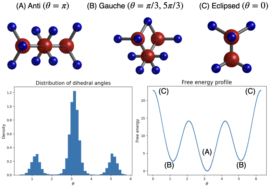
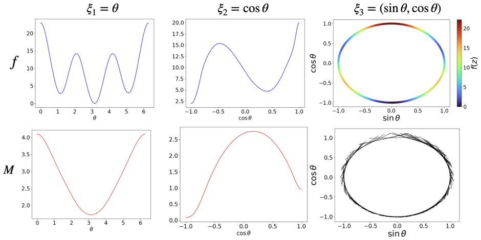
The central claim is that a collective variable satisfying the orthogonality condition $D\xi\nabla V_1 = 0$ reproduces the statistical properties of the original overdamped Langevin dynamics under scale separation, and that this condition is equivalent to the projected orthogonality condition $(I-\Pi)^{\top}\nabla V_1 = 0$. The equivalence means one geometric constraint controls both relative entropy and pathwise error estimates in coarse graining. The paper implements this by learning a surrogate manifold from featurized simulation data, learning a signed-distance surrogate potential on it, and training an encoder whose gradient is orthogonal to the surrogate potential’s gradient; the resulting collective variable is the composition of that encoder with the manifold embedding. In the butane case study, the learned variable separates the anti and gauche states and reproduces the anti-gauche transition rate within ten percent relative error, whereas the conventional dihedral angle overestimates it by 24 percent. The paper further claims that a rank-deficient diffusion tensor—as in the $(\sin\theta, \cos\theta)$ variable—does not prevent faithful transition rates.
Load-bearing premise
The construction assumes the learned surrogate manifold faithfully represents the true residence manifold, with its normal directions matching the true stiff fast directions; if the diffusion-map embedding is distorted, self-intersecting, or mis-dimensioned, the orthogonality condition enforced in latent space need not correspond to the fast subspace of the original dynamics.
Editorial extensions
If this is right
- Transition rates for rare conformational changes can be computed from the low-dimensional effective dynamics once the learned collective variable satisfies the orthogonality condition, avoiding brute-force all-atom simulation.
- The equivalence of (OC) and (POC) means a single constraint improves both relative-entropy and pathwise estimates of coarse-graining error.
- The butane experiments suggest that requiring $D\xi D\xi^{\top}$ to be uniformly positive definite is too strong; rank-deficient diffusion tensors still yield correct rates as long as the collective variable does not collapse distinct metastable states.
- Group-invariant featurization that retains hydrogen coordinates can change the learned manifold enough to make the difference between a collective variable that separates metastable states and one that does not.
Reading between the lines
- The same pipeline should carry over to any molecule whose stiff degrees of freedom produce a codimension-one residence manifold, but only if the feature map yields a topologically faithful embedding; the paper’s own HyperSurface score gives false negatives, so this is the main transfer risk.
- The rank-deficiency evidence invites a theoretical extension: error estimates for effective dynamics with degenerate diffusion tensors, replacing uniform positive definiteness with a weaker condition that the diffusion tensor does not vanish on its support.
- The Laplacian conformal autoencoder’s ability to undo self-intersections is a standalone manifold-learning contribution that could be tested on other spectral embeddings independent of collective-variable construction.
- One testable extension is to compare the feature-map route to Haar-averaged group-invariant diffusion-map kernels on the same butane data, since the paper notes the two routes have not been compared.
Editorial analysis
A structured set of objections, weighed in public.
Referee Report
Summary. The paper revisits quantitative coarse-graining for overdamped Langevin dynamics, proves the equivalence of the orthogonality condition (OC) and the projected orthogonality condition (POC), and proposes a data-driven pipeline (Algorithm 1) for learning collective variables: featurize MD data, embed the residence manifold as a hypersurface via diffusion maps/diffusion nets/LAPCAE, learn a surrogate signed-distance potential, and enforce orthogonality in the latent space. The method is tested on butane, where the PlaneAlign-based CV is reported to reproduce the anti-gauche transition rate at 1.25×10⁻² ps−1 versus the reference 1.13±0.08×10⁻² ps−1. The paper also provides empirical evidence that a rank-deficient diffusion tensor can still reproduce transition rates and emphasizes the role of hydrogen atoms in featurization.
Significance. If the central claim were fully supported, the paper would make a useful contribution: Proposition 2 gives a clean identification of two conditions from different error estimates, the surrogate-manifold framework is a plausible route to imposing geometric conditions without knowing V1, the butane study is detailed, and the code is public. The empirical demonstration with (sin θ, cos θ) showing that a rank-deficient diffusion tensor can reproduce rates is interesting and relevant. However, the quantitative headline claim is contradicted by the authors' own table, and the connection between the latent-space condition actually imposed and the theoretical condition used in the error estimates is not established. The approach is defensible, but the paper currently overstates what is proven and what is demonstrated.
major comments (3)
- [Abstract; §5.4, Table 2] The paper repeatedly claims a 'less than ten percent' relative error for the PlaneAlign CV, but Table 2 gives 1.25×10⁻² ps−1 against the reference 1.13±0.08×10⁻² ps−1. Relative to the point estimate this is (1.25−1.13)/1.13 ≈ 10.6%, slightly above ten percent. The Introduction's phrase 'nearly 10%' is accurate, but the Abstract and §5.4 are not. This is a concrete, checkable numerical claim and should be corrected or carefully qualified (e.g., 'within 1.5 standard deviations of the reference').
- [Algorithm 1; §5.2; §6 (Limitations)] Algorithm 1 enforces the condition ∇bξ·∇bΦ = 0 in latent coordinates, but the theoretical estimates (32) and (40), as well as Proposition 2, concern the true condition Dξ∇V1 = 0 in the all-atom space R^N. For ξ = bξ ∘ Ψ, the chain rule gives Dξ = (Dbξ ∘ Ψ)DΨ, so latent orthogonality controls only the component of DΨ∇V1 aligned with ∇bΦ; no quantitative bound is supplied that transfers the surrogate condition to the true coarse-graining error. The acknowledgment in §6 that (OC) is imposed on the surrogate rather than in R^N does not by itself close this gap. Without such a transfer estimate, the reported PlaneAlign rate improvement cannot be attributed to satisfaction of the advertised orthogonality condition rather than to a favorable reparameterization of the dihedral angle.
- [§4.4; §5.2] The successful case study is selected by visual inspection, and the successful CV is then also chosen by inspection. Section 4.4 states that PlaneAlign 'clearly visually' gives the best 2D embedding despite its low HyperSurface score, and §5.2 sets bξ(x) = arctan2(x2, x1) after observing that the embedding is a circle parameterized by the dihedral angle. This weakens the demonstration that the proposed algorithm automatically discovers a good CV: the favorable result could be obtained by any smooth reparameterization of the dihedral angle. The paper should either present these two choices as human-guided and moderate the claims accordingly, or provide an automated selection criterion that recovers PlaneAlign without visual inspection.
minor comments (4)
- [§3.2.1] The transition rate for ξ3 = (sin θ, cos θ) is printed as '1.19 ps−1' in the text; it should read 1.19×10⁻² ps−1 to match Table 1.
- [§2.2.1] The inequality is attributed to 'Cziszar-Kullback'; the standard spelling is Csiszár-Kullback. The same spelling appears in the proposition label and should be corrected.
- [§4.5; §5.1] The notation 'Leikonal' is used for the eikonal loss in equation (71); consider renaming to 'L_eikonal' for consistency with the rest of the text.
- [Table 3] The header 'F eature map' contains a stray space; also, the table would be easier to read if the hyperparameter column distinguished αZero, αnormals, and αOC explicitly, since αnormals is reported as 0.0 for both rows.
Circularity Check
Latent OC is built into the network by construction, and the PlaneAlign CV is read off from an embedding already parameterized by the dihedral angle; the headline rate is therefore a smooth reparameterization of a known CV.
-
self definitional
[Section 3.3 (Algorithm 1) and Section 6 (Limitations)]
"Finally, we learn bξ which satisfies the (OC) ∇bξ · ∇bΦ = 0. Notably, this bξ can be lifted to an overall collective variable via composition with the parameterization, given by ξ := bξ ◦ Ψ. Therefore, our method can be described as recovering a CV by enforcing the orthogonality condition in a latent space RD+1 instead of the ambient space RN . ... in our framework, the orthogonality condition (OC) is imposed on the surrogate manifold rather than directly in the all-atom space RN ."
The theoretical estimates (32) and (40) require Dξ∇V1 = 0 in the all-atom space RN. Algorithm 1 instead trains ∇bξ·∇bΦ=0, where bΦ is defined as the signed-distance surrogate potential whose gradient is, by construction, the normal to the learned manifold cM. Any bξ orthogonal to that normal satisfies the latent condition automatically, so the statement that the learned CV satisfies (OC) is built into the loss rather than derived from the true fast subspace. The paper explicitly concedes that OC is imposed on the surrogate manifold, not in RN, and provides no estimate transferring latent orthogonality to D(bξ∘Ψ)∇V1.
-
renaming known result
[Section 4.4 and Section 5.2]
"PlaneAlign provides a better embedding than GramMatrixCarbon because the PlaneAlign embedding is a circle parameterized by the dihedral angle ... For PlaneAlign, we find that bξ(x) = arctan2(x2, x1) ... is orthogonal to ∇bΦ and therefore satisfies (OC). Thus, given an interpretable enough visualization, CVs may be devised by inspection. Interestingly, the CV learned via PlaneAlign correlates significantly with the dihedral angle."
The headline CV is selected by inspecting the PlaneAlign diffusion-map embedding after seeing that it is a circle parameterized by the known good CV, the dihedral angle. Setting bξ=arctan2(x2,x1) is reading off the angular coordinate of that circle; Section 5.4 then reports that this CV 'corresponds nearly exactly to the dihedral angle.' The resulting rate 1.25e-2 is therefore a smooth reparameterization of the dihedral-angle CV, whose two-dimensional (sinθ,cosθ) form already gave 1.19e-2 in Table 1. Presenting this as a machine-learned CV that 'reproduces the anti-gauche transition rate' renames a known empirical CV in the new latent coordinates rather than deriving a new prediction from the orthogonality condition.
full rationale
The analytical core is not circular: Proposition 2 proves (OC) ⇔ (POC) algebraically from the SVD of Dξ, and the error estimates (30), (32), (39), (40) are quoted from external prior work. The transition-rate numbers are also benchmarked against an independent brute-force all-atom reference (1.13±0.08×10^-2 ps^-1) and computed by solving the low-dimensional committor BVP with estimated free energies and diffusion tensors, not by fitting to that reference. So this is not a case of the whole derivation collapsing into its inputs. The circularity is partial and localized to the experimental claim. First, the algorithm's central condition is enforced as ∇bξ·∇bΦ=0 on a learned surrogate signed-distance function, making the latent 'OC' true by construction while the paper admits it is not imposed in RN; no transfer bound connects this to the true condition that drives the theory. Second, the PlaneAlign CV used for the headline rate is chosen by inspection after observing that the embedding is parameterized by the known dihedral angle, and arctan2 is essentially that angle, so the rate is a validation of a reparameterized known CV rather than an independent discovery. The paper's own limitation that HyperSurface gives false negatives for the very PlaneAlign embedding later used for the headline rate reinforces that the rate result rests on post-hoc visual selection rather than on the proposed selection heuristic. Note also that the claimed 'less than ten percent relative error' is not met by the reported numbers: 1.25×10^-2 is 10.6% above 1.13×10^-2. No load-bearing self-citation chain was found; the cited same-author items [Cam13], [ECT22], [SEC23] are used for standard rate/diffusion-map numerics and are not invoked to force the CV choice.
Assumptions & free parameters
free parameters (6)
- diffusion map bandwidth epsilon =
tuned via kernel sum test; exact value not reported
- embedding dimension D+1 =
2 or 3 depending on feature map
- number of Laplacian eigenfunctions m =
25
- regularization weight zeta =
0.01
- loss weights alpha_DNet, alpha_LAPCAE, alpha_Zero, alpha_normals, alpha_OC =
1.0, 0.5, 1.0, 0.0, 1.0 (per Table 3)
- transition rate boundary widths =
A = {|θ − π| ≤ 0.2}, B = {|θ − π/3| ≤ 0.1} ∪ {|θ − 5π/3| ≤ 0.1}
assumptions (5)
- domain assumption The featurized trajectory samples a well-defined immersed hypersurface M̂ in RD+1.
- domain assumption The machine-learned diffusion net Ψ approximates the diffusion map embedding faithfully on the full manifold, not only on training points.
- ad hoc to paper The surrogate potential Φ̂ learned from the eikonal loss has gradients that approximate normals to the true residence manifold M.
- domain assumption Langevin dynamics at friction 10 ps−1 is well approximated by the overdamped dynamics (1), and the anisotropic mass rescaling in Appendix A correctly converts rates to physical time units.
- standard math Standard assumptions of the effective dynamics theory: log-Sobolev inequality, Lipschitz drift and diffusion, finite κ, λ.
invented entities (2)
-
Surrogate manifold M̂ with surrogate potential Φ̂
-
LAPCAE (Laplacian Conformal Autoencoder)
Cite this review
Pith. "Pith review of Learning collective variables that preserve transition rates." pith.science (2026). https://pith.science/paper/UONIDIJE
@misc{pith2026250601222,
  author       = {Pith},
  title        = {Pith review of: Learning collective variables that preserve transition rates},
  year         = {2026},
  howpublished = {\url{https://pith.science/paper/UONIDIJE}},
  note         = {Machine review of arXiv:2506.01222}
}
read the original abstract
Collective variables (CVs) play a crucial role in capturing rare events in high-dimensional systems, motivating the continual search for principled approaches to their design. In this work, we revisit the framework of quantitative coarse graining and identify the orthogonality condition from Legoll and Lelievre (2010) as a key criterion for constructing CVs that accurately preserve the statistical properties of the original process. We establish that satisfaction of the orthogonality condition enables error estimates for both relative entropy and pathwise distance to scale proportionally with the degree of scale separation. Building on this foundation, we introduce a general numerical method for designing neural network-based CVs that integrates tools from manifold learning with group-invariant featurization. To demonstrate the efficacy of our approach, we construct CVs for butane and achieve a CV that reproduces the anti-gauche transition rate with less than ten percent relative error. Additionally, we provide empirical evidence challenging the necessity of uniform positive definiteness in diffusion tensors for transition rate reproduction and highlight the critical role of light atoms in CV design for molecular dynamics.
Figures

Figures from the paper (13 more)



Reference graph
Works this paper leans on
-
[1]
Combining docking and molecular dynamic simulations in drug design
[ABG06] Hernan Alonso, Andrey A Bliznyuk, and Jill E Gready. “Combining docking and molecular dynamic simulations in drug design”. In: Medicinal research reviews 26.5 (2006), pp. 531–568.43 Figure 16: Free energy and diffusion tensor for PlaneAlign. 44 [Alt+08] Alex Altis, Martin Otten, Phuong H. Nguyen, Rainer Hegger, and Gerhard Stock. “Dihedral angle p...
work page 2006
-
[2]
Well-tempered metadynamics: a smoothly converging and tunable free-energy method
url: https : / / www . sciencedirect . com / science / article / pii / S1063520314000426. [BBP08] Alessandro Barducci, Giovanni Bussi, and Michele Parrinello. “Well-tempered metadynamics: a smoothly converging and tunable free-energy method”. In: Physical review letters 100.2 (2008), p. 020603. [Bel+23] Zineb Belkacemi, Marc Bianciotto, Herv´ e Minoux, To...
2008
-
[5]
[Mis+19] Gal Mishne, Uri Shaham, Alexander Cloninger, and Israel Cohen. “Diffusion nets”. In: Applied and Computational Harmonic Analysis 47.2 (2019), pp. 259–
work page 2019
-
[285]
tICA-metadynamics: accelerating metadynamics by using kinetically selected collective variables
[MP17] Mohammad M. Sultan and Vijay S Pande. “tICA-metadynamics: accelerating metadynamics by using kinetically selected collective variables”. In: Journal of chemical theory and computation 13.6 (2017), pp. 2440–2447. [M¨ ul+21] Kai R. M¨ uller, Wenkai Zhang, Madhusudhanan Krishnamoorthy, Cecilia Clementi, and Frank No´ e. “Estimating the diffusion tenso...
work page 2017
-
[503]
Diffusion tensors in collective variables spaces: Application to metadynamics
[FP17] Sean A. Fitzgerald and Michele Parrinello. “Diffusion tensors in collective variables spaces: Application to metadynamics”. In: The Journal of Chemi- cal Physics 147.15 (2017), p. 152716. doi: 10.1063/1.4998435. [GKS04] Dror Givon, Raz Kupferman, and Andrew Stuart. “Extracting macroscopic dynamics: model problems and algorithms”. In: Nonlinearity 1...
arXiv 2017
-
[1992]
Towards a theory of transition paths
[EV06] Weinan E and Eric Vanden-Eijnden. “Towards a theory of transition paths”. In: Journal of statistical physics 123.3 (2006), p
work page 2006
-
[2017]
url: https://pure.tue.nl/ws/files/ 51661644/20170112_Sharma.pdf. [SK11] Vojtˇ ech Spiwok and Blanka Kr´ alov´ a. “Metadynamics in the conformational space nonlinearly dimensionally reduced by Isomap”. In: The Journal of chem- ical physics 135.22 (2011). [SMH23] Subarna Sasmal, Martin McCullagh, and Glen M Hocky. “Reaction coordinates for conformational tr...
work page Pith review arXiv 2011
-
[2131]
Pathwise estimates for an ef- fective dynamics
[LLO17] Fr´ ed´ eric Legoll, Tony Leli` evre, and Stefano Olla. “Pathwise estimates for an ef- fective dynamics”. In: Stochastic Processes and their Applications 127.9 (2017), pp. 2841–2863. [LLS19] Fr´ ed´ eric Legoll, Tony Leli` evre, and Upanshu Sharma. “Effective dynamics for non-reversible stochastic differential equations: a quantitative study”. In:...
work page 2017
Show all 11 references
-
[4517]
Computing committors via Mahalanobis diffusion maps with enhanced sampling data
[ECT22] Luke Evans, Maria K Cameron, and Pratyush Tiwary. “Computing committors via Mahalanobis diffusion maps with enhanced sampling data”. In:The Journal of Chemical Physics 157.21 (2022). [EG92] L.C. Evans and R.F. Gariepy. Measure Theory and Fine Properties of Func- tions....
2022
-
[4779]
Pathwise estimates for effective dynamics: The case of nonlinear vectorial reaction coordinates
[LZ19a] T. Leli` evre and W. Zhang. “Pathwise estimates for effective dynamics: The case of nonlinear vectorial reaction coordinates”. In: Multiscale Modeling & Simulation 17.3 (2019), pp. 1019–1051. doi: 10.1137/18M1216793. [LZ19b] Tony Leli` evre and Wei Zhang. “Pathwise est...
2019 doi
-
[6338]
Fast recovery of free energy landscapes via diffusion-map-directed molecular dynamics
[PC14] Jordane Preto and Cecilia Clementi. “Fast recovery of free energy landscapes via diffusion-map-directed molecular dynamics”. In: Physical Chemistry Chem- ical Physics 16.36 (2014), pp. 19181–19191. [P´ er+13] Guillermo P´ erez-Hern´ andez, Fabian Paul, Toni Giorgino, Gi...
2014 arXiv
Reviewed August 7, 2026 · model on record in the stance chip above.
Discussion (0). Sign in to comment.