REVIEW 2 major objections 6 minor 38 references
Long-time asymptotics of the defocusing mKdV equation with step initial data
T0 review · 2 major / 6 minor · reviewed 2026-08-07 · deepseek-v4-flash
Pith's one-line read The paper proves that for $q_r\ge q_l\ge 0$ the long-time solution of the defocusing mKdV equation with step initial data splits into three zones, with the central dispersive shock described by a modulated Jacobi elliptic wave fixed by a…
desk verdict Theorem 1.1's central Region II elliptic formula is inconsistent with the paper's own Appendix A (wrong sign of V) and with its Appendix C derivation (factor of 2 in Vt). read the letter →
The pith
A machine-rendered reading of the paper's core claim, the machinery that carries it, and where it could break.
The reading
What carries the argument
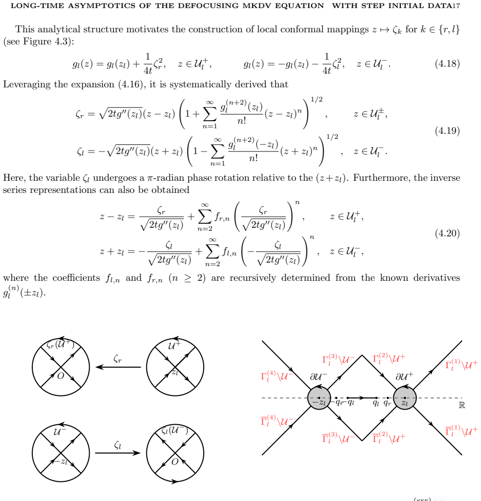
The argument runs through the Riemann–Hilbert problem for the mKdV Lax pair, renormalized by a $g$-function chosen on a hyperelliptic curve of genus zero, two, or zero according to the region. The load-bearing object is the genus-two $g$-function $g_d(\xi;z)$ of (5.1), whose branch points are the Riemann invariants $(q_l,z_d,q_r)$; the condition that the differential vanish at the soft edge $z_d$ yields the Whitham velocity equation $12\xi=v_1(q_l,z_d,q_r)$. The paper generalizes a conformal-transformation genus reduction to pass from the genus-two model problem to a genus-one Riemann–$\theta$ function, and the reconstruction formula is then evaluated with Jacobi $\theta$ and elliptic identities to give (1.12). The scalar functions $D_l$ and $D_d$ absorb the continuous-spectrum data and produce the phase shifts and prefactors of the asymptotic formulas.
What would settle it
Take $q_l=0.2$, $q_r=0.8$, and $t=200$; extract the local oscillation wavelength and amplitude from a direct numerical solution across the dispersive shock zone, then compare with (1.12) using $z_d(\xi)$ computed by solving (5.2). If the pointwise difference does not decay like $t^{-1}$, or if (5.2) has two roots for some $\xi$ in Region II, Theorem 1.1's central claim is false.
Extended reading notes
Core claim
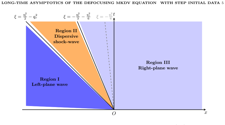
The paper proves Theorem 1.1: for $q_r\ge q_l\ge 0$, the long-time solution of the defocusing mKdV equation with step initial data has three asymptotically distinct regimes. In Region I, determined by the ray $\xi=x/(12t)$, the solution approaches the left background $q_l$ with a $t^{-1/2}$ oscillatory correction whose phase contains a logarithmic shift. In Region III it approaches the right background $q_r$ exponentially fast. The central assertion is Region II: on an intermediate ray interval the solution is, up to $O(t^{-1})$, a modulated Jacobi elliptic wave $q_{\mathrm{dsw}}(x,t)$ of the explicit form in (1.12), with velocity $V=q_l^2+q_r^2+z_d^2$ and elliptic modulus $m^2=(q_r^2-z_d^2)/(q_r^2-q_l^2)$, where the modulation parameter $z_d(\xi)$ is determined by the Whitham velocity equation (5.2)–(5.3). Thus the dispersive shock zone is exactly a slowly varying elliptic traveling wave.
Load-bearing premise
The central formula for the dispersive shock zone presumes that the equation fixing the modulation parameter, $12\xi=v_1(q_l,z_d,q_r)$, has a unique solution $z_d(\xi)$ throughout Region II; the paper relies on strict monotonicity of this Whitham velocity, a property imported from known strict hyperbolicity of the KdV Whitham equations rather than proved here.
Editorial extensions
If this is right
- If Theorem 1.1 holds, a dispersive shock wave generated by a step is a deterministic modulated elliptic wave whose velocity and modulus are fixed by the initial heights $q_l$ and $q_r$ through the Whitham equation.
- The dispersive shock zone occupies rays $x/(12t)$ between $q_l^2/2-q_r^2$ and $-q_l^2/3-q_r^2/6$, so the zone expands linearly in time.
- When $q_l=0$, the general formulas collapse to an explicit modulated cnoidal wave and to the classical oscillatory asymptotics for rapidly decaying data, checking the construction against a known limit.
- In the right region, convergence to $q_r$ is exponentially fast, so the right background is approached with no oscillatory tail.
- The paper's numerical comparisons at $t=15$ for $(q_l,q_r)=(0,0.5)$ and $(0.2,0.8)$ agree with the leading-order formulas, supporting the claim that the asymptotic regime is visible at moderate time.
Reading between the lines
- Not in the paper: the same $g$-function machinery could be pushed into the two narrow transition layers at the edges of the dispersive shock zone, which the paper explicitly leaves out.
- Not in the paper: for $q_r<0$ the paper notes that an additional kink-soliton region appears, so extending Theorem 1.1 to signed steps would require adding a discrete-spectrum contribution to the modulated elliptic wave.
- Not in the paper: because the paper's relation (5.4) connects its Whitham velocity to the KdV Whitham velocity, the modulation parameter $z_d(\xi)$ could be computed from existing KdV shock-tube data and compared with direct mKdV numerics as an independent check.
Editorial analysis
A structured set of objections, weighed in public.
Referee Report
Summary. This paper studies the long-time asymptotics of the defocusing mKdV equation (1.1) with step initial data (1.2) in the regime q_r ≥ q_l ≥ 0. The authors set up the associated Riemann-Hilbert problem, construct genus-zero and genus-two g-functions, and apply the Deift-Zhou nonlinear steepest descent method with Airy and parabolic-cylinder local parametrices. Theorem 1.1 claims three asymptotic regimes: a left plane-wave region with an oscillatory t^{-1/2} correction, a central dispersive shock wave region described by a modulated Jacobi elliptic wave q_dsw, and a right plane-wave region with exponential convergence to q_r. The paper also provides a numerical comparison at t = 15.
Significance. If correct, the result would be an important rigorous characterization of dispersive shock waves for the defocusing mKdV equation with step data, extending the Deift-Zhou framework beyond decaying initial data. The derivation is parameter-free: the scattering data are computed from the initial step, the modulation parameter z_d is fixed by (5.2)-(5.3), and the numerics are used only as post hoc verification. The g-function construction and the genus-two-to-genus-one reduction are carried out in detail. The main caveats are the internal inconsistencies in the central elliptic formula described below, the fact that the two transition strips are excluded, and the qualitative nature of the numerical comparison.
major comments (2)
- [§1.1, Eq. (1.12)-(1.13); Appendix A, Eq. (A.9)-(A.10); §5, Eq. (5.16); Appendix C, Eq. (C.16)] The stated traveling-wave velocity in the central Region II formula is incorrect by a factor of two, and the phase sign in (1.12) is not reconciled with Appendix A. For the roots in (A.8), the coefficient V in the ODE (A.2)-(A.3) equals Σ_{i<k} q_i q_k = -2(z_1^2+z_2^2+z_3^2). With the ansatz φ=x−Vt used in Appendix A, the exact periodic solution (A.9) therefore has argument x+2(z_1^2+z_2^2+z_3^2)t, not x−(z_1^2+z_2^2+z_3^2)t. The paper, however, sets V=z_1^2+z_2^2+z_3^2 in (A.10) and (1.13), so the displayed q_dsw in (1.12) is not the exact traveling wave solution it is claimed to be. This is load-bearing because q_dsw is the leading-order term of Theorem 1.1. The paper's own RHP calculation supports the factor 2: (5.16) gives δ0 proportional to x+2(q_l^2+q_r^2+z_d^2)t, and the final expression in (C.16) therefore has this phase. Theorem 1.1 and Remark 1.1 should be restated with V=2(q_l^2+q_r^2+z_d^2) together with the plus sign, or with an equivalent correction in the sign convention of Appendix A.
- [§5, after Eq. (5.5); Theorem 1.1; Remark 1.1] The justification of the modulation parameter z_d does not formally cover the case q_l=0, although this case is included in Theorem 1.1 and treated in Remark 1.1. The text states that (5.3) is invertible 'only when z_d >0 or equivalently when q_l >0'. For q_l=0, the open interval z_d∈(0,q_r) still has z_d>0, so the intended Implicit Function Theorem argument can be made to work, but it is not made. The paper should state that invertibility holds on the open interval z_d∈(q_l,q_r) and that the limiting endpoints are approached as m→1 and m→0. As written, the proof appears to exclude the q_l=0 case it claims to cover.
minor comments (6)
- [Appendix A, Eq. (A.8)] The formula for q4 is printed as z2+z3−z2, which is identical to z3; it should presumably be z2+z3−z1, consistent with the roots used elsewhere.
- [Appendix A, Eq. (A.10)] The expression V=z1^2+z2^2+z3^3 contains a typo (z3^3 instead of z3^2); moreover, in light of Major Comment 1 the numerical factor is incorrect.
- [§5, Eq. (5.8)] The identifications 'm→0 (or z_d→q_l)' and 'm→1 (or z_d→q_r)' are reversed, since m^2=(q_r^2−z_d^2)/(q_r^2−q_l^2); m→0 corresponds to z_d→q_r and m→1 corresponds to z_d→q_l.
- [§5, Eq. (5.2)] The displayed integral appears as ∫_{q_r}^{z_d}; the intended interval and orientation (presumably from z_d to q_r) should be stated explicitly.
- [Figure 1.4] The numerical validation is carried out at t=15 only and no error estimate is provided; the phrase 'perfect agreement' overstates the evidence.
- [Remark 1.1] The attribution of the q_l=0 plane-wave formula to Deift-Zhou [12] for rapidly decaying initial data should be qualified, since the present setting is step-like initial data.
Circularity Check
No circularity found: the long-time asymptotics are derived from the Riemann-Hilbert analysis with parameters fixed by the initial data, not by the target solution.
full rationale
The derivation chain is self-contained. The scattering data r(z), a(z) are computed explicitly from the step initial data in (2.16)-(2.17). The g-functions are constructed from the spectral geometry (Section 3) and the branch point z_d in Region II is fixed by equation (5.2), which is the self-similarity/soft-edge condition (3.11) and is shown to be uniquely solvable via equation (5.5) using Levermore's strict hyperbolicity theorem for KdV Whitham equations [29]—an external, independent result. The leading-order elliptic wave (1.12) is then obtained by solving the model RHP 5.2 via the theta-function construction (5.31) and the conformal change of variables (5.32); no parameter is fitted to the target solution or to numerical data. The numerical simulations are used only as post hoc verification (Figure 1.4), not to set any constants. There is no self-citation chain that carries the argument, and the cited results ([12,17,21,29]) are independent. A separate sign discrepancy between the phase in (1.12) and Appendix A (x-x0+Vt vs x-x0-Vt) is a potential correctness issue, but it is not a circular step: it does not involve defining a quantity in terms of the target result or fitting a parameter to the predicted quantity.
Assumptions & free parameters
assumptions (5)
- standard math Strict hyperbolicity of the KdV Whitham modulation equations and the relation v1(z1,z2,z3)=w(-z3^2,-z2^2,-z1^2) imply d(v1)/d(z2) < 0, giving a unique z_d via the implicit function theorem.
- domain assumption The Cauchy problem (1.1)-(1.2) is well-posed under the integrability condition (1.3), and the scattering coefficient a(z) has no zeros when q_r >= q_l >= 0, so no solitons appear.
- standard math Vanishing lemma for Schwartz-symmetric Riemann-Hilbert problems ensures existence and uniqueness of the solution to RHP 2.1.
- standard math Deift-Zhou steepest descent, Beals-Coifman small-norm theory, and the standard parabolic cylinder and Airy model solutions are valid and applicable to the RHPs constructed here.
- domain assumption The initial data are restricted to q_r >= q_l >= 0; the paper explicitly excludes the cases q_r < q_l and the sign combinations that generate kink solitons.
Cite this review
Pith. "Pith review of Long-time asymptotics of the defocusing mKdV equation with step initial data." pith.science (2026). https://pith.science/paper/Z4GSHCEH
@misc{pith2026250601570,
  author       = {Pith},
  title        = {Pith review of: Long-time asymptotics of the defocusing mKdV equation with step initial data},
  year         = {2026},
  howpublished = {\url{https://pith.science/paper/Z4GSHCEH}},
  note         = {Machine review of arXiv:2506.01570}
}
read the original abstract
This work investigates the long-time asymptotics of solution to defocusing modified Korteweg-de Vries equation with a class of step initial data. A rigorous asymptotic analysis is conducted on the associated Riemann-Hilbert problem by applying Deift-Zhou nonlinear steepest descent method. In this process, the construction of odd-symmetry g-function is generalized and the method of genus reduction on the Riemann-theta function is proposed via conformal transformation and symmetries. It is revealed that for sufficiently large time, the solution manifests a tripartite spatiotemporal structure, i.e., in the left plane-wave region, the solution decays to a modulated plane wave with oscillatory correction; in the central dispersive shock wave region, the solution is governed by a modulated elliptic periodic wave; in the right plane wave region, the solution converges exponentially to a constant. The results from the long-time asymptotic analysis have been shown to match remarkably well with that obtained by direct numerical simulations.
Figures


Figures from the paper (9 more)




Reference graph
Works this paper leans on
-
[1]
M. J. Ablowitz, D. J. Kaup, A. C. Newell, H. Segur, Nonlinear-Evolution Equations of Physical Significance, Phys. Rev. Lett. 31 (2) (1973) 125-127
work page 1973
-
[2]
M. J. Ablowitz, H. Segur, Asymptotic Solutions of the Korteweg-deVries Equation, Stud. Appl. Math. 57 (1) (1977) 13-44
work page 1977
-
[3]
K. Andreiev, I. Egorova, T. L. Lange, G. Teschl, Rarefaction waves of the Korteweg–de Vries equation via nonlinear steepest descent, J. Differ. Equ. 261 (10) (2016) 5371-5410
work page 2016
- [4]
-
[5]
M. Bertola, A. Minakov, Laguerre polynomials and transitional asymptotics of the modified Korte- weg–de Vries equation for step-like initial data, Anal. Math. Phys. 9 (4) (2019) 1761-1818
work page 2019
-
[6]
G. Biondini, S. T. Li, D. Mantzavinos, Long-Time Asymptotics for the Focusing Nonlinear Schr¨ odinger Equation with Nonzero Boundary Conditions in the Presence of a Discrete Spectrum, Commun. Math. Phys. 382 (2021) 1495-1577
work page 2021
-
[7]
A. Boutet de Monvel, A. Its, V. Kotlyarov, Long-Time Asymptotics for the Focusing NLS Equation with Time-Periodic Boundary Condition on the Half-Line, Commun. Math. Phys. 290 (2009) 479- 522
work page 2009
-
[8]
A. Boutet de Monvel, V. P. Kotlyarov, D. Shepelsky, Focusing NLS Equation: Long-Time Dynamics of Step-Like Initial Data, Int. Math. Res. Not. 2011 (7) (2011) 1613–1653
work page 2011
Show all 38 references
-
[9]
Boutet de Monvel, J
A. Boutet de Monvel, J. Lenells, D. Shepelsky, The Focusing NLS Equation with Step-Like Os- cillating Background: Scenarios of Long-Time Asymptotics, Commun. Math. Phys. 383 (2) (2021) 893-952
2021
-
[10]
Buckingham, S
R. Buckingham, S. Venakides, Long-time asymptotics of the nonlinear Schr¨ odinger equation shock problem, Comms. Pure Appl. Math. 60 (9) (2007) 1349-1414
2007
-
[11]
Cuccagna and R
S. Cuccagna and R. Jenkins, On the Asymptotic Stability ofN-Soliton Solutions of the Defocusing Nonlinear Schr¨ odinger Equation, Commun. Math. Phys. 343 (2016) 921-969
2016
-
[12]
Deift, X
P. Deift, X. Zhou, A steepest descent method for oscillatory Riemann-Hilbert problems. Asymptotics for the MKdV equation, Ann. of Math. 137 (2) (1993) 295-368
1993
-
[13]
C. F. Driscoll, T. M. O’Neil, Modulational instability of cnoidal wave solutions of the modified Korteweg–de Vries equation, J. Math. Phys. 17 (7) (1976) 1196-1200
1976
-
[14]
Egorova, Z
I. Egorova, Z. Gladka, V. Kotlyarov, G. Teschl, Long-time asymptotics for the Korteweg–de Vries equation with step-like initial data, Nonlinearity 26 (2013) 1839
2013
-
[15]
G. A. El, M. A. Hoefer, M. Shearer, Dispersive and diffusive-dispersive shock waves for nonconvex conservation laws, SIAM Review, 59 (2017) 3-61
2017
-
[16]
Fromm, J
S. Fromm, J. Lenells, R. Quirchmayr, The defocusing nonlinear Schr¨ odinger equation with step-like oscillatory initial data, Adv. Diff. Equations, 30 (2025) 455-525
2025
-
[17]
Grava, A
T. Grava, A. Minakov, On the Long-Time Asymptotic Behavior of the Modified Korteweg–de Vries Equation with Step-like Initial Data, SIAM J. Math. Anal. 52 (6) (2020) 5892-5993
2020
-
[18]
Grava, F
T. Grava, F. R. Tian, The generation, propagation, and extinction of multiphases in the KdV zero- dispersion limit, Comm. Pure Appl. Math. 55 (12) (2002) 1569-1639
2002
-
[19]
A. V. Gurevich, L. P. Pitaevskii, Decay of Initial Discontinuity in the Korteweg-de Vries Equation, Sov. J. Exp. Theor. Phys. Lett. 17 (1973) 193
1973
-
[20]
K. R. Helfrich, W. K. Melville, J. W. Miles, On interfacial solitary waves over slowly varying topog- raphy, J. Fluid Mech. 149 (1984) 305-317
1984
-
[21]
Jenkins, Regularization of a sharp shock by the defocusing nonlinear Schr¨ odinger equation, Non- linearity 28 (7) (2015) 2131
R. Jenkins, Regularization of a sharp shock by the defocusing nonlinear Schr¨ odinger equation, Non- linearity 28 (7) (2015) 2131
2015
-
[22]
Kakutani, N
T. Kakutani, N. Yamasaki, Solitary Waves on a Two-Layer Fluid, J. Phys. Soc. Jpn. 45 (2) (1978) 674-679. LONG-TIME ASYMPTOTICS OF THE DEFOCUSING MKDV EQUA TION WITH STEP INITIAL DA T A41
1978
-
[23]
A. M. Kamchatnov, A. Spire, V. V. Konotop, On dissipationless shock waves in a discrete nonlinear Schr¨ odinger equation, J. Phys. A: Math. Gen. 37 (2004) 5547-5568
2004
-
[24]
E. Ya. Khruslov, Asymptotics of the solution of the Cauchy problem for the Korteweg–de Vries equation with initial data of step type, Math. USSR-Sb. 28 (2) (1976) 229-248
1976
-
[25]
Kotlyarov, A
V. Kotlyarov, A. Minakov, Riemann–Hilbert problem to the modified Korteveg–de Vries equation: Long-time dynamics of the steplike initial data, J. Math. Phys. 51 (9) (2010) 093506
2010
-
[26]
Kotlyarov, A
V. Kotlyarov, A. Minakov, Step-Initial Function to the MKdV Equation: Hyper-Elliptic Long-Time Asymptotics of the Solution, J. Math. Phys. Anal. Geom. 8 (1) (2012) 38–62
2012
-
[27]
Kotlyarov, A
V. Kotlyarov, A. Minakov, Modulated elliptic wave and asymptotic solitons in a shock problem to the modified Korteweg-de Vries equation, J. Math. Anal. Appl. 48 (1) (2015) 81-104
2015
-
[28]
V. P. Kotlyarov, E. Ya. Khruslov, Asymptotic solitons of the modified Korteweg-de Vries equation, Inverse Problems 5 (6) (1989) 1075
1989
-
[29]
C. D. Levermore, The hyperbolic nature of the zero dispersion Kdv limit, Commun. Partial Differ- ential Equations 13 (4) (1988) 495-514
1988
-
[30]
Minakov, Asymptotics of step-like solutions for the Camassa–Holm equation J
A. Minakov, Asymptotics of step-like solutions for the Camassa–Holm equation J. Differ. Equ. 261 (11) (2016) 6055-6098
2016
-
[31]
R. M. Miura, Korteweg-de Vries Equation and Generalizations. I. A Remarkable Explicit Nonlinear Transformation, J. Math. Phys. 9 (8) (1968) 1202-1204
1968
-
[32]
N. I. Muskhelishvili, Singular Integral Equations: Boundary Problems of Functions Theory and Their Applications to Mathematical Physics, Wolters-Noordhoff (1958)
1958
-
[33]
Rybalko, D
Y. Rybalko, D. Shepelsky, Curved wedges in the long-time asymptotics for the integrable nonlocal nonlinear Schr¨ odinger equation, Stud. Appl. Math. 147 (3) (2021) 872-903
2021
-
[34]
Tajiri, K
M. Tajiri, K. Nishihara, Solitons and Shock Waves in Two-Electron-Temperature Plasmas, J. Phys. Soc. Jpn. 54 (1985) 572-578
1985
-
[35]
Watanabe, Ion Acoustic Soliton in Plasma with Negative Ion, J
S. Watanabe, Ion Acoustic Soliton in Plasma with Negative Ion, J. Phys. Soc. Jpn. 53 (3) (1984) 950-956
1984
-
[36]
Xu, On the large-time asymptotics of the defocusing mKdV equation with step-like initial data, arXiv:2204.01299
T.Y. Xu, On the large-time asymptotics of the defocusing mKdV equation with step-like initial data, arXiv:2204.01299
-
[37]
V. E. Zakharov, S. V. Manakov, Asymptotic behavior of non-linear wave systems integrated by the inverse scattering method, Zh. Eksp. Teor. Fiz. 71 (1) (1976) 203
1976
-
[38]
Zhou, The Riemann–Hilbert Problem and Inverse Scattering, SIAM J
X. Zhou, The Riemann–Hilbert Problem and Inverse Scattering, SIAM J. Math. Anal. 20 (4) (1989) 966-986. Deng-Shan W ang: Laboratory of Mathematics and Complex Systems (Ministry of Education), School of Mathematical Sciences, Beijing Normal University, Beijing 100875, China Ema...
1989
Reviewed August 7, 2026 · model on record in the stance chip above.
Discussion (0). Sign in to comment.