REVIEW 3 major objections 5 minor 1 cited by
Rootin' Tootin' Efficient Ray Shootin': Creating Microlensing Magnification Maps with GPUs
T0 review · 3 major / 5 minor · reviewed 2026-08-07 · deepseek-v4-flash
Pith's one-line read The fastest publicly available microlensing map generator combines GPU parallelization, the fast multipole method, and inverse polygon mapping to cut map-making from CPU hours to GPU minutes.
desk verdict A credible, useful GPU microlensing map generator with convincing external validation, but the FMM error control in extreme-magnification regimes and the 'fastest' headline both need more support. read the letter →
The pith
A machine-rendered reading of the paper's core claim, the machinery that carries it, and where it could break.
The reading
What carries the argument
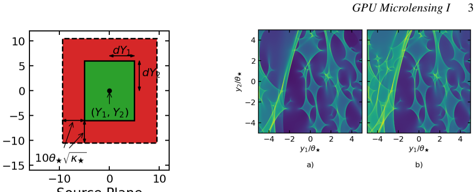
The load-bearing machinery is a GPU-accelerated fast multipole method (FMM) tree combined with inverse polygon mapping (IPM). The FMM builds a quadtree over the image plane; for each ray the deflection from the at most 32 microlenses in the ray's own node and its neighbors is summed directly, while all farther microlenses are represented by a Taylor series whose coefficients come from multipole-to-local translations, reducing the per-ray work from a sum over all $N_\star$ lenses to a sum over a bounded number of nearby lenses plus a polynomial of order at most 31. The expansion order is chosen from a single-mass truncation error bound so that the series converges to a deflection-accuracy target of one-tenth of a pixel side. IPM replaces ray counting: each cell of the image-plane grid is mapped to the source plane, split into two triangles, clipped against pixel boundaries with the Sutherland-Hodgman algorithm, and each clipped area is added to the pixel it covers, so Poisson noise from ray counts is avoided. The paper also derives the image-plane region that must be shot, using the cross-correlation of the source-plane rectangle with the microlens deflection-angle PDF, which adds a $\kappa_\star$- and mass-spectrum-dependent border before macromodel inversion.
What would settle it
Generate one extreme-magnification map twice with identical microlens positions, masses, and pixel grid: once with the fast multipole method at the default expansion order and once with direct summation over every microlens. If any pixel's magnification differs by more than the accuracy implied by the one-tenth-pixel deflection target in dense caustic regions, or if the discrepancies grow systematically as the stellar density increases, then the symmetry-cancellation assumption fails and the claimed speed-to-accuracy tradeoff is not uniformly safe.
Extended reading notes
Core claim
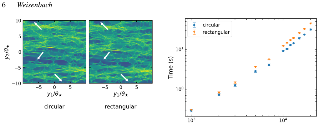
On its own terms, this paper establishes that the combination of GPU execution, the fast multipole method, and inverse polygon mapping reduces the cost of microlensing magnification maps far below the current public state of the art. For a fixed $20\theta_\star \times 20\theta_\star$ map at 2000 by 2000 pixels with roughly 27,000 circularly distributed microlenses, the paper reports 0.763 seconds with the fast multipole method and inverse polygon mapping, versus 39.367 seconds without the multipole method and 348.884 seconds for direct inverse ray shooting; with rectangular microlens regions the fastest time rises slightly to 0.839 seconds. For an extreme-magnification case near a cluster caustic, the paper reports map generation in about 200 to 600 seconds in single and double precision, compared with roughly 30 CPU-hours quoted for similar simulations, and finds the runtime to be essentially independent of the number of microlenses up to $\sim10^8$. Accuracy is checked by comparing light curves and magnification histograms with an existing CPU inverse-polygon tool, finding agreement within a few percent, and by internal consistency checks that find no differences between maps with and without the fast multipole method or between inverse polygon mapping and inverse ray shooting.
Load-bearing premise
The speed and accuracy of the fast maps rest on the assumption that the error from cutting off the distant-star approximation stays small when many distant groups of stars are summed, relying on errors from opposite sides to cancel by symmetry; the paper tests this only by comparing its fast maps with its own direct maps, not with an analytic guarantee of the accumulated error.
Editorial extensions
If this is right
- Magnification maps for survey-scale parameter studies can be produced in seconds to minutes on one GPU, rather than hours on CPU clusters, making broad parameter scans practical.
- Because runtime is essentially independent of the number of microlenses up to $\sim10^8$, high-stellar-density environments such as galaxy cluster cores become computationally accessible at high resolution.
- Light curves and magnification histograms from the fast maps agree with those from a CPU inverse-polygon tool to within a few percent, so the speedup does not come at the cost of visibly changed statistics.
- The code handles a range of microlens mass spectra and both circular and rectangular microlens regions; with the FMM active, the rectangular region no longer speeds up map generation because its smooth-sheet deflection angle is more expensive.
Reading between the lines
- (Editorial inference) If the runtime scales as reported, time-dependent microlensing with moving stars and systematic scans over the microlens mass spectrum become practical at parameter-space scales that were previously too expensive; the paper names these as future applications but does not quantify the resulting cost reduction.
- (Editorial inference) The single-precision artifacts in the extreme-magnification section point toward a mixed-precision strategy or shifting coordinates to the map center before computing deflections; the paper documents the artifacts but does not propose these remedies.
- (Editorial inference) Because the FMM error argument leans on symmetric cancellation of truncation errors, a direct pixel-level comparison of FMM and direct summation across a grid of $\kappa_\star$ values would test whether the default expansion order is safe in the densest caustic networks.
Editorial analysis
A structured set of objections, weighed in public.
Referee Report
Summary. This manuscript presents RooTERS, a CUDA-based microlensing magnification-map generator that combines a fast multipole method (FMM) for the stellar deflection with inverse polygon mapping (IPM) for pixel apportionment. The code is validated against the independent online tool gloton.ugr.es at one parameter set (κ=κ★=γ=0.6), where light curves agree within about 1% and magnification histograms are essentially identical, and against internal FMM-on/off and IPM/IRS consistency checks. Timing benchmarks on an NVIDIA A100 show weak dependence on the number of microlenses up to ~10^8 and roughly quadratic scaling with pixel count, with map generation times of seconds to minutes in several configurations. The paper also demonstrates the method in extreme-magnification cluster-lensing settings and documents substantial single-precision artifacts, recommending double precision there.
Significance. The contribution is practically significant for the microlensing community: if the FMM accuracy is properly controlled, the code provides a public tool that can generate high-resolution maps in minutes rather than CPU-hours, enabling large parameter surveys and studies of lensed quasars, supernovae, and cluster-crossing stars. Genuine strengths include the public repository, validation against an independently published online tool and the standard analytic lens equation, repeated timing runs with standard deviations, and careful treatment of the image-plane boundary and mass-spectrum effects. The main risk is the unquantified FMM error in exactly the extreme-magnification regime that the paper showcases, where caustic positions are highly sensitive to small deflection errors.
major comments (3)
- [§4.1 and Appendix C3 (Eqs. C8–C9)] The FMM expansion-order criterion is the load-bearing accuracy control of the method, but Eq. (C8) is a single-mass, single-distant-node bound and Eq. (C9) is justified by a symmetry-cancellation heuristic that the paper itself calls 'not a perfect error estimate.' The internal FMM-on/off check in Section 4.1 reports that no differences are found without specifying a quantitative tolerance, and the external validation covers a single parameter set (κ=κ★=γ=0.6). In the Section 5 extreme-magnification maps, where |1−κ−γ|^{-1}=1000 makes caustic locations highly sensitive to small deflection errors, the maps are produced with the FMM only. I find this concern valid and load-bearing: the largest speedups are claimed precisely in the regime where the FMM error is least tested. I request either a quantitative FMM-on/off comparison at the Section 5 parameters (e.g., per-ray deflection errors or map-level caustic offsets), or a many-node error bound that does not rely on unverified cancellation, together with a stated tolerance for 'no differences.'
- [§4.2, Fig. 7, Table 1] The headline claim of being 'the fastest microlensing map generation code currently publicly available' is supported only by comparisons with GPU-D, a 2010-generation GPU code, and a CPU implementation of IPM. The manuscript acknowledges these are not like-for-like comparisons, but the abstract states the claim without that qualification. Since speed is the paper's central advertised contribution, the authors should benchmark against a current GPU implementation of a comparable method on the same A100, or explicitly separate algorithmic speedup from hardware-driven improvement in the abstract and conclusions. As written, the 'orders of magnitude' statement conflates the two.
- [§5, Figs. 8–12] The single-precision analysis convincingly shows that double precision is required for extreme-magnification configurations, but the double-precision maps themselves are not independently validated in this regime. The only checks are against the noisier single-precision maps and the single κ=κ★=γ=0.6 external comparison. Because Section 5 is presented as a demonstration of the code's capability in the regime where the FMM speedups matter most, I recommend adding an independent reference for at least one small patch of a double-precision extreme map (e.g., a direct-sum or FMM-off calculation on a subregion), or explicitly stating that this accuracy test remains future work.
minor comments (5)
- [§1] The text 'Whileteralens (Alpay 2019)' appears to be missing a space; it should read 'While teralens'.
- [§3.2] The 'Sutherland-Cohen algorithm' is more commonly called the 'Cohen-Sutherland algorithm'; please correct the name or define the variant used.
- [§4.1 and Figs. 4–5] For reproducibility, please specify the precise metric behind 'essentially indistinguishable' histograms (e.g., a Kolmogorov–Smirnov statistic or maximum fractional difference) and the exact fraction of light-curve points within the 1% band.
- [§6] The statement that 'There are no remaining improvements that could significantly reduce the computational runtime required outside of altering the code to run on multiple GPUs' is too strong, given the acknowledged approximate quadratic scaling with pixel count; please soften it.
- [Data availability] Please provide a versioned release or commit hash (and ideally a DOI via Zenodo) for the repository, so the published benchmarks are reproducible when the code evolves.
Circularity Check
No significant circularity: the code is validated against independently published online tools and the standard lens equation, with speed claims based on benchmarks rather than derived from fitted inputs.
full rationale
The paper's central claims are computational: it implements FMM and IPM on GPUs and benchmarks runtimes. No parameter is fitted to make a prediction succeed, and no claimed output is defined in terms of the quantity it purports to predict. The magnification accuracy is checked against maps and microlens fields downloaded from the independently published online tool gloton.ugr.es (Jiménez-Vicente & Mediavilla 2022) and against direct IRS-without-FMM calculations in an internal consistency check (Section 4.1), while the lens equation (Eq. 7) is the standard physical input rather than a consequence of the code's output. The Appendix C3 error bound (Eq. C8) is quoted from Petersen et al. (1995) and is explicitly described as 'not a perfect error estimate' when many distant nodes contribute, with a symmetry-cancellation heuristic leading to Eq. C9; this is an accuracy caveat about an approximation, not a circular step, and the speed claim is benchmark-based rather than derived from that bound. The only self-reference is an 'in prep.' pointer to separate critical-curve work, which is not load-bearing for the map-generation results. No self-definitional relation, fitted-input-called-prediction pattern, imported uniqueness theorem, or renamed known result appears in the derivation chain.
Assumptions & free parameters
free parameters (4)
- Maximum microlenses directly used per node =
32
- Maximum Taylor series order =
31
- Deflection accuracy target =
1/10 of pixel side length
- PDF tail fraction f =
1/1000 (default)
assumptions (5)
- domain assumption Lens potential can be Taylor expanded to second order with higher derivatives negligible
- domain assumption Microlens deflection PDF tail behaves as p(|alpha'|) = theta^2 kappa <m^2>/(pi |alpha'|^4 <m>)
- standard math FMM multipole and local expansion formulas of Greengard and Rokhlin apply to gravitational lensing
- domain assumption Errors from many distant FMM nodes cancel by symmetry
- domain assumption Rectangular and circular microlens regions produce equivalent statistics
Cite this review
Pith. "Pith review of Rootin' Tootin' Efficient Ray Shootin': Creating Microlensing Magnification Maps with GPUs." pith.science (2026). https://pith.science/paper/NPRFM2SO
@misc{pith2026250602114,
  author       = {Pith},
  title        = {Pith review of: Rootin' Tootin' Efficient Ray Shootin': Creating Microlensing Magnification Maps with GPUs},
  year         = {2026},
  howpublished = {\url{https://pith.science/paper/NPRFM2SO}},
  note         = {Machine review of arXiv:2506.02114}
}
read the original abstract
The impending discovery and monitoring of hundreds of new gravitationally lensed quasars and supernovae from upcoming ground and space based large area surveys such as LSST, \textit{Euclid}, and \textit{Roman} necessitates the development of improved numerical methods for studying gravitational microlensing. We present in this work the fastest microlensing map generation code currently publicly available. We utilize graphics processing units to take advantage of the inherent parallelizable nature of creating magnification maps, in addition to using 1) the fast multipole method to reduce the runtime dependence on the number of microlenses and 2) inverse polygon mapping to reduce the number of rays required. The code is available at https://github.com/weisluke/microlensing/.
Figures


Figures from the paper (8 more)




Forward citations
Cited by 1 Pith paper
-
Microlensing of Microlensing: Effects of Random Stars on the Double-Source-Plane Gravitational Lens
First numerical ray-shooting simulation of compound (two-plane) quasar microlensing in the double-source-plane lens J1721+8842 shows new caustic morphologies — convexity violations and lip caustics — that do not occur...
Reference graph
Works this paper leans on
-
[1]
Alpay A., 2019, https://github.com/illuhad/teralens
work page 2019
-
[2]
Barnes J., Hut P., 1986, @doi [ ] 10.1038/324446a0 , https://ui.adsabs.harvard.edu/abs/1986Natur.324..446B 324, 446
doi:10.1038/324446a0 1986
-
[3]
Bate N. F., Fluke C. J., Barsdell B. R., Garsden H., Lewis G. F., 2010, @doi [ ] 10.1016/j.newast.2010.05.008 , https://ui.adsabs.harvard.edu/abs/2010NewA...15..726B 15, 726
-
[4]
Bourassa R. R., Kantowski R., 1975, @doi [ ] 10.1086/153300 , https://ui.adsabs.harvard.edu/abs/1975ApJ...195...13B 195, 13
doi:10.1086/153300 1975
-
[5]
Bourassa R. R., Kantowski R., Norton T. D., 1973, @doi [ ] 10.1086/152452 , https://ui.adsabs.harvard.edu/abs/1973ApJ...185..747B 185, 747
doi:10.1086/152452 1973
-
[6]
Carrier J., Greengard L., Rokhlin V., 1988, @doi [SIAM Journal on Scientific and Statistical Computing] 10.1137/0909044 , 9, 669
doi:10.1137/0909044 1988
-
[7]
New Approximation of Magnification Statistics for Random Microlensing of Magnified Sources
Dai L., Pascale M., 2021, @doi [arXiv e-prints] 10.48550/arXiv.2104.12009 , https://ui.adsabs.harvard.edu/abs/2021arXiv210412009D p. arXiv:2104.12009
work page Pith review arXiv doi:10.48550/arxiv.2104.12009 2021
-
[8]
Diego J. M., 2019, @doi [ ] 10.1051/0004-6361/201833670 , https://ui.adsabs.harvard.edu/abs/2019A&A...625A..84D 625, A84
Show all 47 references
-
[9]
M., 2022, @doi [ ] 10.1051/0004-6361/202244027 , https://ui.adsabs.harvard.edu/abs/2022A&A...665A.127D 665, A127
Diego J. M., 2022, @doi [ ] 10.1051/0004-6361/202244027 , https://ui.adsabs.harvard.edu/abs/2022A&A...665A.127D 665, A127
2022 doi
-
[10]
M., et al., 2018, @doi [ ] 10.3847/1538-4357/aab617 , https://ui.adsabs.harvard.edu/abs/2018ApJ...857...25D 857, 25
Diego J. M., et al., 2018, @doi [ ] 10.3847/1538-4357/aab617 , https://ui.adsabs.harvard.edu/abs/2018ApJ...857...25D 857, 25
2018 doi
-
[11]
D., Treu T., Marshall P., Liao K., Hojjati A., Linder E., Rumbaugh N., 2015, @doi [ ] 10.1088/0004-637X/799/2/168 , https://ui.adsabs.harvard.edu/abs/2015ApJ...799..168D 799, 168
Dobler G., Fassnacht C. D., Treu T., Marshall P., Liao K., Hojjati A., Linder E., Rumbaugh N., 2015, @doi [ ] 10.1088/0004-637X/799/2/168 , https://ui.adsabs.harvard.edu/abs/2015ApJ...799..168D 799, 168
2015 doi
-
[12]
A., Heydenreich S., 2020, @doi [ ] 10.3847/1538-4357/abbdf7 , https://ui.adsabs.harvard.edu/abs/2020ApJ...904..176E 904, 176
Esteban-Guti \'e rrez A., Ag \"u es-Paszkowsky N., Mediavilla E., Jim \'e nez-Vicente J., Mu \ n oz J. A., Heydenreich S., 2020, @doi [ ] 10.3847/1538-4357/abbdf7 , https://ui.adsabs.harvard.edu/abs/2020ApJ...904..176E 904, 176
2020 doi
-
[13]
F., 2010, @doi [ ] 10.1016/j.newast.2009.06.006 , https://ui.adsabs.harvard.edu/abs/2010NewA...15..181G 15, 181
Garsden H., Lewis G. F., 2010, @doi [ ] 10.1016/j.newast.2009.06.006 , https://ui.adsabs.harvard.edu/abs/2010NewA...15..181G 15, 181
2010 doi
-
[14]
Greengard L., Rokhlin V., 1987, @doi [Journal of Computational Physics] 10.1016/0021-9991(87)90140-9 , https://ui.adsabs.harvard.edu/abs/1987JCoPh..73..325G 73, 325
1987 doi
-
[15]
Jim \'e nez-Vicente J., Mediavilla E., 2022, @doi [ ] 10.3847/1538-4357/ac9e59 , https://ui.adsabs.harvard.edu/abs/2022ApJ...941...80J 941, 80
2022 doi
-
[16]
Katz N., Balbus S., Paczynski B., 1986, @doi [ ] 10.1086/164313 , https://ui.adsabs.harvard.edu/abs/1986ApJ...306....2K 306, 2
1986 doi
-
[17]
Kayser R., Refsdal S., Stabell R., 1986, , https://ui.adsabs.harvard.edu/abs/1986A&A...166...36K 166, 36
1986
-
[18]
R., 2001, @doi [arXiv e-prints] 10.48550/arXiv.astro-ph/0102340 , https://ui.adsabs.harvard.edu/abs/2001astro.ph..2340K pp astro--ph/0102340
Keeton C. R., 2001, @doi [arXiv e-prints] 10.48550/arXiv.astro-ph/0102340 , https://ui.adsabs.harvard.edu/abs/2001astro.ph..2340K pp astro--ph/0102340
-
[19]
L., et al., 2018, @doi [Nature Astronomy] 10.1038/s41550-018-0430-3 , https://ui.adsabs.harvard.edu/abs/2018NatAs...2..334K 2, 334
Kelly P. L., et al., 2018, @doi [Nature Astronomy] 10.1038/s41550-018-0430-3 , https://ui.adsabs.harvard.edu/abs/2018NatAs...2..334K 2, 334
2018 doi
-
[20]
S., 2004, @doi [ ] 10.1086/382180 , https://ui.adsabs.harvard.edu/abs/2004ApJ...605...58K 605, 58
Kochanek C. S., 2004, @doi [ ] 10.1086/382180 , https://ui.adsabs.harvard.edu/abs/2004ApJ...605...58K 605, 58
2004 doi
-
[21]
A., Lopez P., Mediavilla T., Abajas C., Gonzalez-Morcillo C., Gil-Merino R., 2006, @doi [ ] 10.1086/508796 , https://ui.adsabs.harvard.edu/abs/2006ApJ...653..942M 653, 942
Mediavilla E., Mu \ n oz J. A., Lopez P., Mediavilla T., Abajas C., Gonzalez-Morcillo C., Gil-Merino R., 2006, @doi [ ] 10.1086/508796 , https://ui.adsabs.harvard.edu/abs/2006ApJ...653..942M 653, 942
2006 doi
-
[22]
A., Ariza O., Lopez P., Gonzalez-Morcillo C., Jimenez-Vicente J., 2011, @doi [ ] 10.1088/0004-637X/741/1/42 , https://ui.adsabs.harvard.edu/abs/2011ApJ...741...42M 741, 42
Mediavilla E., Mediavilla T., Mu \ n oz J. A., Ariza O., Lopez P., Gonzalez-Morcillo C., Jimenez-Vicente J., 2011, @doi [ ] 10.1088/0004-637X/741/1/42 , https://ui.adsabs.harvard.edu/abs/2011ApJ...741...42M 741, 42
2011 doi
-
[23]
K., Arad O., Zitrin A., 2022, @doi [ ] 10.1093/mnras/stac1511 , https://ui.adsabs.harvard.edu/abs/2022MNRAS.514.2545M 514, 2545
Meena A. K., Arad O., Zitrin A., 2022, @doi [ ] 10.1093/mnras/stac1511 , https://ui.adsabs.harvard.edu/abs/2022MNRAS.514.2545M 514, 2545
2022 doi
-
[24]
Neindorf B., 2003, @doi [ ] 10.1051/0004-6361:20030098 , https://ui.adsabs.harvard.edu/abs/2003A&A...404...83N 404, 83
2003 doi
-
[25]
M., Kaiser N., Kelly P
Oguri M., Diego J. M., Kaiser N., Kelly P. L., Broadhurst T., 2018, @doi [ ] 10.1103/PhysRevD.97.023518 , https://ui.adsabs.harvard.edu/abs/2018PhRvD..97b3518O 97, 023518
2018 doi
-
[26]
M., Diego J
Palencia J. M., Diego J. M., Kavanagh B. J., Mart \' nez-Arrizabalaga J., 2024, @doi [ ] 10.1051/0004-6361/202347492 , https://ui.adsabs.harvard.edu/abs/2024A&A...687A..81P 687, A81
2024 doi
-
[27]
G., Soelvason D., Perram J
Petersen H. G., Soelvason D., Perram J. W., Smith E. R., 1995, Proceedings: Mathematical and Physical Sciences, 448, 389
1995
-
[28]
O., Rider B., Teguia A
Petters A. O., Rider B., Teguia A. M., 2009, @doi [Journal of Mathematical Physics] 10.1063/1.3158854 , https://ui.adsabs.harvard.edu/abs/2009JMP....50g2503P 50, 072503
2009 doi
-
[29]
Refsdal S., Stabell R., 1991, , https://ui.adsabs.harvard.edu/abs/1991A&A...250...62R 250, 62
1991
-
[30]
Schneider P., Weiss A., 1986, , https://ui.adsabs.harvard.edu/abs/1986A&A...164..237S 164, 237
1986
-
[31]
Schneider P., Weiss A., 1987, , https://ui.adsabs.harvard.edu/abs/1987A&A...171...49S 171, 49
1987
-
[32]
E., 1992, Gravitational Lenses , @doi 10.1007/978-3-662-03758-4
Schneider P., Ehlers J., Falco E. E., 1992, Gravitational Lenses , @doi 10.1007/978-3-662-03758-4
1992 doi
-
[33]
Seitz C., Schneider P., 1994, , https://ui.adsabs.harvard.edu/abs/1994A&A...288....1S 288, 1
1994
-
[34]
N., Gil-Merino R., Goicoechea L
Shalyapin V. N., Gil-Merino R., Goicoechea L. J., 2021, @doi [ ] 10.1051/0004-6361/202140527 , https://ui.adsabs.harvard.edu/abs/2021A&A...653A.121S 653, A121
2021 doi
-
[35]
E., Hodgman G
Sutherland I. E., Hodgman G. W., 1974, @doi [Commun. ACM] 10.1145/360767.360802 , 17, 32–42
1974
-
[36]
C., Fluke C
Thompson A. C., Fluke C. J., Barnes D. G., Barsdell B. R., 2010, @doi [ ] 10.1016/j.newast.2009.05.010 , https://ui.adsabs.harvard.edu/abs/2010NewA...15...16T 15, 16
2010 doi
-
[37]
Venumadhav T., Dai L., Miralda-Escud \'e J., 2017, @doi [ ] 10.3847/1538-4357/aa9575 , https://ui.adsabs.harvard.edu/abs/2017ApJ...850...49V 850, 49
2017 doi
-
[38]
J., 2013, @doi [ ] 10.1093/mnras/stt1076 , https://ui.adsabs.harvard.edu/abs/2013MNRAS.434..832V 434, 832
Vernardos G., Fluke C. J., 2013, @doi [ ] 10.1093/mnras/stt1076 , https://ui.adsabs.harvard.edu/abs/2013MNRAS.434..832V 434, 832
2013 doi
-
[39]
J., 2014, @doi [Astronomy and Computing] 10.1016/j.ascom.2014.05.002 , https://ui.adsabs.harvard.edu/abs/2014A&C.....6....1V 6, 1
Vernardos G., Fluke C. J., 2014, @doi [Astronomy and Computing] 10.1016/j.ascom.2014.05.002 , https://ui.adsabs.harvard.edu/abs/2014A&C.....6....1V 6, 1
2014 doi
-
[40]
J., Bate N
Vernardos G., Fluke C. J., Bate N. F., Croton D., 2014, @doi [ ] 10.1088/0067-0049/211/1/16 , https://ui.adsabs.harvard.edu/abs/2014ApJS..211...16V 211, 16
2014 doi
-
[41]
Wambsganss J., 1990, PhD thesis, -
1990
-
[42]
Wambsganss J., 1999, Journal of Computational and Applied Mathematics, https://ui.adsabs.harvard.edu/abs/1999JCoAM.109..353W 109, 353
1999
-
[43]
Welch B., et al., 2022, @doi [ ] 10.1038/s41586-022-04449-y , https://ui.adsabs.harvard.edu/abs/2022Natur.603..815W 603, 815
2022 doi
-
[44]
J., 1990, , https://ui.adsabs.harvard.edu/abs/1990A&A...236..311W 236, 311
Witt H. J., 1990, , https://ui.adsabs.harvard.edu/abs/1990A&A...236..311W 236, 311
1990
-
[45]
Wyithe J. S. B., Webster R. L., 1999, @doi [ ] 10.1046/j.1365-8711.1999.02515.x , https://ui.adsabs.harvard.edu/abs/1999MNRAS.306..223W 306, 223
1999
-
[46]
Yang X.-L., Chen X.-C., Zheng W.-W., Luo Y., 2023, @doi [ ] 10.1016/j.chinastron.2023.09.005 , https://ui.adsabs.harvard.edu/abs/2023ChA&A..47..570Y 47, 570
2023 doi
-
[47]
Zheng W., Chen X., Li G., Chen H.-Z., 2022, @doi [ ] 10.3847/1538-4357/ac68ea , https://ui.adsabs.harvard.edu/abs/2022ApJ...931..114Z 931, 114
2022 doi
Reviewed August 7, 2026 · model on record in the stance chip above.
Discussion (0). Sign in to comment.