REVIEW 4 major objections 5 minor 76 references
Temporal horizons in forecasting: a performance-learnability trade-off
T0 review · 4 major / 5 minor · reviewed 2026-08-07 · deepseek-v4-flash
Pith's one-line read Longer training horizons make the loss landscape exponentially rougher for chaotic systems and linearly rougher for limit cycles, while long-horizon minima still generalize better to short horizons.
desk verdict A promising framework for horizon selection whose headline theorems are not yet proven as stated—the O/Omega gap is real and load-bearing; still worth a serious referee. read the letter →
The pith
A machine-rendered reading of the paper's core claim, the machinery that carries it, and where it could break.
The reading
What carries the argument
The load-bearing object is the $\varepsilon$-bounded region: a convex set of parameters inside which the model's one-step Jacobian $J_f(x,\theta)$ stays within $\varepsilon^2$ of the true system Jacobian $J_\phi(x)$ for every state $x$. Lemma A.6 shows that inside such a region the model Jacobian converges to the true Jacobian, so the system's Lyapunov exponent $\lambda$ (the rate at which nearby trajectories separate) or cycle frequency $\omega$ is inherited by the products of state-space Jacobians $J_x^\tau(x,\theta)=\prod_{k=1}^{\tau} J_x(f^k(x),\theta)$ that appear in the chain-rule expansion of the loss gradient. That product, growing like $e^{\lambda\tau}$ for chaos and like $\omega\tau$ for limit cycles, is what carries the scaling from the dynamics into the gradient, the Hessian, and the roughness of the landscape. The $\varepsilon$-bounded region is also the boundary condition of the theory: the results apply only to partially trained models whose parameters stay in such a region, not to models at initialization.
What would settle it
Train an autoregressive MLP on a chaotic system and, at each checkpoint, measure both the relative gradient norm $g(T)$ and whether the current parameters satisfy the $\varepsilon$-bounded-region condition $\|f(x+\varepsilon r,\theta)-(f(x,\theta)+J_\phi(x)\varepsilon r)\|<\varepsilon^2$ on a sample of states. If $g(T)$ fails to grow like $e^{\lambda T}$ whenever the condition holds, or if it grows exponentially while the condition is violated, the causal link from system dynamics to loss-landscape geometry is broken. A complementary check: for connected minima of the losses at $T_l$ and $T_h$, the transfer ratio should track $e^{\lambda(T_h-T_l)}$; sweeping a system parameter to vary $\lambda$ over a factor of ten and confirming the rate would settle whether the exponential constant is really the Lyapunov exponent.
Extended reading notes
Core claim
On its own terms, the paper's central discovery is that the geometry of an autoregressive forecasting loss is not a property of the model alone: it inherits the temporal signature of the underlying dynamical system. The paper shows that the relative gradient norm $g(T) = \|\nabla_\theta L(\theta,T)\|/\|\nabla_\theta L(\theta,1)\|$ scales as $O(e^{\lambda T})$ for chaotic or locally unstable systems and as $O(\omega T)$ for limit cycles, with the same scaling inherited by the Hessian around minima and by the number of extrema along any line in parameter space. The minima found at different horizons are asymmetric in their transfer: a minimum found at a long horizon $T_h$ performs well when evaluated at a short horizon $T_l$, while the reverse fails with the same exponential or linear factor, so long-horizon minima capture the global dynamics better. The paper also proves that as $T\to\infty$ the loss surface becomes a fractal, which would make gradient descent fail entirely. Together these results imply that single-step training and training exactly at the evaluation horizon are both suboptimal defaults.
Load-bearing premise
The whole argument assumes the trained model has already learned the dynamics well enough that its local behavior matches the real system's local behavior across the whole region of parameter space that training visits; only under that alignment do the system's divergence rate or cycle speed transfer to the model's gradients and produce the predicted scalings.
Editorial extensions
If this is right
- Single-step training ($T=1$) is not a safe default: a model trained one step ahead suffers exponentially (chaotic systems) or linearly (periodic systems) worse error when used for long-horizon forecasts.
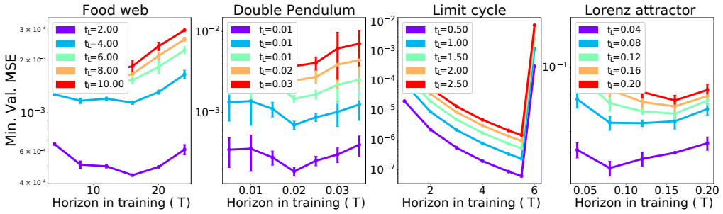
- The optimal training horizon is a U-shaped function of $T$; in the paper's experiments on the Lorenz attractor, double pendulum, food web, limit cycle, and two climate benchmarks, it never coincides with the evaluation horizon.
- More compute shifts the optimum toward longer horizons: with a fixed wall-clock budget, splitting training across increasing horizons outperforms any single fixed horizon.
- For perfectly known mechanistic models with an identifiable zero-loss solution, the long-horizon generalization advantage disappears and the smallest $T$ wins; the trade-off reappears once noise or model misspecification is introduced.
- As $T\to\infty$ the loss landscape becomes fractal and non-differentiable, so no gradient-based optimizer can train an infinite-horizon forecaster, regardless of architecture.
Reading between the lines
- The theorems imply that the dimensionless product $\lambda T$ (or $\omega T$), not $T$ alone, is the real control parameter: two chaotic systems with different Lyapunov exponents should need proportionally scaled training horizons. This is a quantitative prediction the paper does not state, and a parameter sweep across $\lambda$ could test it directly.
- The same Jacobian-product mechanism should apply to any composition length in an autoregressive pipeline, not just forecasting horizons: context length in sequence models, rollout length in model-based control, and multi-token prediction targets in language models likely face the same trade-off. The paper draws these analogies but does not claim the mechanism extends to them.
- The asymmetry of the generalization theorem doubles as a diagnostic: if the measured transfer ratio between long- and short-horizon minima does not grow like $e^{\lambda(T_h-T_l)}$, the model has left the regime the theory describes, telling the practitioner that the model is too far from the true dynamics for the scaling argument to apply.
Editorial analysis
A structured set of objections, weighed in public.
Referee Report
Summary. This paper studies how the training horizon T affects the loss landscape of autoregressive neural network forecasters for deterministic dynamical systems. The authors introduce an 'epsilon-bounded region' of parameter space in which the model Jacobian is close to the true system Jacobian, and from this they derive scaling laws for the loss gradient (Theorem 4.2), the Hessian at minima (Corollary 4.3), a cross-horizon generalization ratio (Theorem 4.4), and the number of extrema along a parameter-space segment (Theorem 4.5). These quantities are claimed to grow exponentially in T for chaotic systems and linearly for limit cycles, implying a U-shaped relationship between training horizon and achievable validation performance. The paper supports the theory with experiments on the Lorenz attractor, a double pendulum, a limit cycle, a food web, and two climate datasets, and it discusses an adaptive horizon-selection heuristic.
Significance. The question addressed is practically important and under-theorized, and the empirical demonstration of U-shaped validation curves across several systems is a useful contribution. The theoretical scaffolding is attractive: the Lyapunov-based mechanism is a natural quantity to examine, and the paper is explicit about its smoothness, ergodicity, and data-quality assumptions. However, the central theorems as written prove only upper bounds where the verbal claims require lower bounds (O versus Ω/Θ), and the key Jacobian-alignment condition is assumed rather than verified in the experiments. The manuscript is therefore not yet at the level of rigor claimed in the abstract, though the core idea may be repairable. No code is provided at this stage, so the numerical experiments are not independently checkable.
major comments (4)
- [§4.3, Theorem 4.5 and §A.13] The conclusion that the number of extrema z(T) grows with T is not established by the proof, because Lemma A.12 requires a lower bound on the total variation v_T = ∫ |∂_l L(l,T)| dl exceeding 2n L_max^ε, while the only quantitative input invoked, Theorem 4.2/A.9, is an upper bound O(e^{λT}) (or O(ωT)) on the normalized gradient. An upper bound on the integrand does not imply that v_T diverges: the gradient magnitude could be large only on a set of measure zero, or could be O(e^{λT}) at one point but small elsewhere, leaving z(T) bounded. The proof needs a lower bound of order e^{λT} for |∂_l L| on a positive-measure subset of the segment, or a direct lower bound on v_T. As written, the theorem should be rephrased as an upper bound, which would not support the abstract's 'exponentially rough landscape' claim.
- [§4.2, Theorem 4.4 and §A.11] The abstract and Section 4.2 interpret Theorem 4.4 as showing that short-horizon minima 'suffer exponentially worse' long-term predictions, but the theorem only states r(Th,Tl) = O(e^{λ(Th−Tl)}) (resp. O(ω(Th−Tl))). An upper bound on the ratio of loss differences is compatible with r being of order one or smaller; the claimed asymmetry requires r to be exponentially (resp. linearly) large, i.e., a lower bound. The proof in A.11 integrates ||∇L(θ,T)|| along the gradient path and again uses only the upper bound from Theorem 4.2. Without an additional lower-bound argument, the generalization claim is not proven.
- [Definition 4.1 and Lemma A.6] The mechanism driving all the scaling results is assumed rather than derived. Lemma A.6 shows that within an epsilon-bounded region the model Jacobian converges to the system Jacobian, but this is essentially a restatement of Definition 4.1 in the limit; it does not prove that training trajectories remain in such a region. The experiments in Figures 1–3 measure g(T) and z(T) during training but do not verify that the parameters visited lie in an epsilon-bounded region, so they do not test the key hypothesis. The theorems should be presented as conditional on the epsilon-bounded-region assumption, and the empirical section should either check the condition or provide a robustness argument for trained models.
- [Theorem A.9, Eqs. (20)–(21)] The derivation of the gradient-growth bound contains an unproven inequality: it assumes ||x(k+τ)−f^τ(x(k),θ)|| ≥ ||x(k+1)−f(x(k),θ)|| for all k and τ, and then drops the J_theta terms using M ≫ T. For models that are already accurate at horizon one, the τ-step error need not dominate the one-step error, and for chaotic systems with good short-time tracking the inequality may fail. If this is intended as a heuristic or an additional assumption, it should be stated as such; Theorem 4.2 inherits this step, so it is load-bearing for all subsequent results.
minor comments (5)
- [§B.3] The section heading 'Pood web model' contains a typo; it should be 'Food web model'.
- [§1] In the introductory paragraph, 'we examine the practical implications' begins with a lowercase 'we' after a period; the capitalization should be fixed.
- [Theorems 4.2, 4.4, 4.5] Theorems that claim growth use big-O notation, which denotes an upper bound; for growth statements the notation should be Ω or Θ unless the claims are explicitly weakened to upper bounds. This is related to the major comments, but even in the statements it misleads the reader.
- [Corollary A.14] The claim that the loss surface becomes a fractal as T→∞ is supported only by a heuristic sentence about 'unbounded gradients' and a space-filling curve; a box-counting argument is not supplied. The corollary should be labeled as a conjecture or given a rigorous proof.
- [Corollary 4.3 and §A.10] The proof identifies the trace of the Hessian with the nuclear norm; these coincide only when the Hessian is positive semidefinite, which is not guaranteed away from the minimum. The corollary should either justify semidefiniteness on the ball or use the nuclear norm consistently.
Circularity Check
Central claims reduce partly by construction: the exponential rate is the defining Lyapunov limit applied under an assumed Jacobian-matching region, and long-to-short generalization is an identity of the nested loss (eq. 3).
-
self definitional
[Theorem 4.2 proof sketch, Section 4.1; Definition 4.1; Lemma A.6]
"Furthermore, within theorem 4.1, the Jacobian of the model remains close to the Jacobian of the true system (theorem A.6). The Jacobian of the model is always contained in the expression for ∇θLx(θ, T), and thus it scales with T."
Definition 4.1 defines the ε-bounded region by requiring the model's local linearization to match Jφ, and Lemma A.6 'proves' Jacobian convergence by Taylor-expanding that same definition. Theorem 4.2's proof then attributes the gradient's T-scaling entirely to this pre-installed Jacobian agreement, while the exponential rate is the defining Lyapunov limit of the true system. The prediction g(T)=O(e^{λT}) is thus the hypothesis 'θ lies in an ε-bounded region' plus the definition of λ, delivered through the chain rule; no independent mechanism is derived. The later roughness and Hessian results inherit this scaling, so the central quantitative claims are not tested independently of the defining assumption.
-
self definitional
[Equation (3); Theorem 4.4 and its proof sketch, Section 4.2]
"Intuitively, the theorem reflects the fact that long temporal predictions rely on shorter predictions, implying that models that are able to make predictions over long temporal horizons must also make good predictions over short time horizons."
Because eq. (3) defines L(θ,T) as an average over τ=1..T, the loss at horizon Tl is, up to normalization, the partial sum of the same per-step errors that enter the loss at horizon Th. Consequently, any parameter with small L(·,Th) automatically has controlled L(·,Tl); the long-to-short generalization asymmetry asserted in Theorem 4.4 and the abstract is an identity of the nested loss definition, not a dynamical discovery. The exponential factor in eq. (8) is then imported from Theorem 4.2, so the qualitative direction of Theorem 4.4 is already contained in the construction of the training loss.
full rationale
The paper contains no load-bearing self-citation: references such as [10] and [50] are contextual and do not justify the main theorems. However, two central theoretical steps are substantially definitional. Definition 4.1 installs Jacobian agreement as the defining property of the ε-bounded region; Lemma A.6 converts that definition into a convergence lemma; and Theorem 4.2 then reads off the Lyapunov exponent's defining growth rate from the model Jacobian product. Separately, the long-horizon loss in eq. (3) is a superset of the short-horizon loss, so the claimed 'long generalizes to short' asymmetry is forced by the loss definition. The numerical experiments (Figs. 1, 3, 5, 6 and the NOAA/ClimSim benchmarks) are genuine external evidence and give the paper independent content, which prevents a maximal score. A further formal gap, flagged here rather than as circularity, is that Theorem 4.5/A.13 uses Lemma A.12, whose hypothesis is a lower bound on total variation v_T, while Theorem 4.2 provides only an O upper bound; as written the proof does not establish that z(T) grows. That is a correctness concern, not a circular reduction. Overall, the headline trade-off is partly forced by construction: the exponential scalings are the defining Lyapunov limit applied under an assumption that already asserts the needed Jacobian tracking, and the generalization benefit is inscribed in the nested loss.
Assumptions & free parameters
free parameters (2)
- epsilon (epsilon-bounded region tolerance)
- Algorithm 1 hyperparameters gamma, eta_0 =
gamma = 1.5e-4; eta_0 user-set
assumptions (6)
- domain assumption The dynamical system is ergodic, stationary, deterministic, and fully observable (Markovian).
- domain assumption The loss is smooth (gradient descent applies); neurons use Softplus rather than ReLU.
- ad hoc to paper Within the epsilon-bounded region, the model Jacobian equals the system Jacobian (Lemma A.6).
- ad hoc to paper The two minima in Theorem 4.4 lie in each other's basin of attraction, and the gradient path between them remains inside an epsilon-bounded region.
- ad hoc to paper For the gradient ratio in Theorem A.9, ||x(k+tau)-f^tau(x(k),theta)|| >= ||x(k+1)-f(x(k),theta)|| and M >> T, allowing J_theta terms to be dropped.
- domain assumption The state space is bounded and the system has a stationary distribution for the loss to be bounded.
Cite this review
Pith. "Pith review of Temporal horizons in forecasting: a performance-learnability trade-off." pith.science (2026). https://pith.science/paper/SC562PGR
@misc{pith2026250603889,
  author       = {Pith},
  title        = {Pith review of: Temporal horizons in forecasting: a performance-learnability trade-off},
  year         = {2026},
  howpublished = {\url{https://pith.science/paper/SC562PGR}},
  note         = {Machine review of arXiv:2506.03889}
}
read the original abstract
When training autoregressive models to forecast dynamical systems, a critical question arises: how far into the future should the model be trained to predict? Too short a horizon may miss long-term trends, while too long a horizon can impede convergence due to accumulating prediction errors. In this work, we formalize this trade-off by analyzing how the geometry of the loss landscape depends on the training horizon. We prove that for chaotic systems, the loss landscape's roughness grows exponentially with the training horizon, while for limit cycles, it grows linearly, making long-horizon training inherently challenging. However, we also show that models trained on long horizons generalize well to short-term forecasts, whereas those trained on short horizons suffer exponentially (resp. linearly) worse long-term predictions in chaotic (resp. periodic) systems. We validate our theory through numerical experiments and discuss practical implications for selecting training horizons. Our results provide a principled foundation for hyperparameter optimization in autoregressive forecasting models.
Figures


Figures from the paper (9 more)



Reference graph
Works this paper leans on
-
[1]
Anna ˚Akesson, Alva Curtsdotter, Anna Ekl¨ of, Bo Ebenman, Jon Norberg, and Gy¨ orgy Barab´ as. The importance of species interactions in eco-evolutionary community dynamics under climate change.Nature Communications, 12(1):4759, 2021
work page 2021
-
[2]
Preferential Temporal Difference Learning
Nishanth Anand and Doina Precup. Preferential temporal difference learning.arXiv preprint arXiv:2106.06508, 2021
work page Pith review arXiv 2021
-
[3]
Unitary evolution recurrent neural networks
Martin Arjovsky, Amar Shah, and Yoshua Bengio. Unitary evolution recurrent neural networks. InInternational conference on machine learning, pp. 1120–1128. PMLR, 2016
work page 2016
-
[4]
Ozgur Aydogmus and Ali Hakan Tor. A modified multiple shooting algorithm for parameter estimation in odes using adjoint sensitivity analysis.Applied Mathematics and Computation, 390:125644, 2021
work page 2021
-
[5]
Benjamin Erichson, Vanessa Lin, and Michael Mahoney
Omri Azencot, N. Benjamin Erichson, Vanessa Lin, and Michael Mahoney. Forecasting sequential data using consistent koopman autoencoders. In Hal Daum´ e III and Aarti Singh (eds.),Proceedings of the 37th International Conference on Machine Learning, volume 119 ofProceedings of Machine Learning Research, pp. 475–485. PMLR, 13–18 Jul 2020. URLhttps://proceed...
work page 2020
-
[6]
Learning long-term dependencies with gradient descent is difficult.IEEE transactions on neural networks, 5(2):157–166, 1994
Yoshua Bengio, Patrice Simard, and Paolo Frasconi. Learning long-term dependencies with gradient descent is difficult.IEEE transactions on neural networks, 5(2):157–166, 1994
1994
-
[7]
Coupled predator–prey oscillations in a chaotic food web.Ecology letters, 12(12):1367–1378, 2009
Elisa Beninc` a, Klaus D J¨ ohnk, Reinhard Heerkloss, and Jef Huisman. Coupled predator–prey oscillations in a chaotic food web.Ecology letters, 12(12):1367–1378, 2009
work page 2009
-
[8]
Dawid Bernaciak and Jim E Griffin. A loss discounting framework for model averaging and selection in time series models.International Journal of Forecasting, 2024. 10
work page 2024
Show all 76 references
-
[9]
Numerical treatment of inverse problems in chemical reaction kinetics
Hans Georg Bock. Numerical treatment of inverse problems in chemical reaction kinetics. InModelling of Chemical Reaction Systems: Proceedings of an International Workshop, Heidelberg, Fed. Rep. of Germany, September 1–5, 1980, pp. 102–125. Springer, 1981
1980
-
[10]
Partitioning time series to improve process-based models with machine learning.bioRxiv, 2024
Victor Boussange, Pau Vilimelis Aceituno, Frank Sch¨ afer, and Lo ¨ ıc Pellissier. Partitioning time series to improve process-based models with machine learning.bioRxiv, 2024. doi: 10.1101/2022.07.25.501365. URL https://www.biorxiv.org/content/early/2024/04/11/2022.07.25.501365
2024 doi
-
[11]
Cambridge university press, 2002
Michael Brin and Garrett Stuck.Introduction to dynamical systems. Cambridge university press, 2002
2002
-
[12]
Antisymmetricrnn: A dynamical system view on recurrent neural networks.arXiv preprint arXiv:1902.09689, 2019
Bo Chang, Minmin Chen, Eldad Haber, and Ed H Chi. Antisymmetricrnn: A dynamical system view on recurrent neural networks.arXiv preprint arXiv:1902.09689, 2019
1902 arXiv
-
[13]
Learning to plan for language modeling from unlabeled data.arXiv preprint arXiv:2404.00614, 2024
Nathan Cornille, Marie-Francine Moens, and Florian Mai. Learning to plan for language modeling from unlabeled data.arXiv preprint arXiv:2404.00614, 2024
2024 arXiv
-
[14]
Bifurcations in the learning of recurrent neural networks 3.learning (RTRL), 3:17, 1992
Kenji Doya et al. Bifurcations in the learning of recurrent neural networks 3.learning (RTRL), 3:17, 1992
1992
-
[15]
Springer, 2008
Gerald A Edgar and Gerald A Edgar.Measure, topology, and fractal geometry, volume 2. Springer, 2008
2008
-
[16]
Roland England.Some Examples of Parameter Estimation by Multiple Shooting, pp. 122–136. Birkh¨ auser Boston, Boston, MA, 1983. ISBN 978-1-4684-7324-7. doi: 10.1007/978-1-4684-7324-7 8. URL https://doi.org/10. 1007/978-1-4684-7324-7_8
1983 doi
-
[17]
Benjamin Erichson, Michael Muehlebach, and Michael W
N. Benjamin Erichson, Michael Muehlebach, and Michael W. Mahoney. Physics-informed autoencoders for lyapunov-stable fluid flow prediction, 2019
2019
-
[18]
Lipschitz recurrent neural networks.arXiv preprint arXiv:2006.12070, 2020
N Benjamin Erichson, Omri Azencot, Alejandro Queiruga, Liam Hodgkinson, and Michael W Mahoney. Lipschitz recurrent neural networks.arXiv preprint arXiv:2006.12070, 2020
2006 arXiv
-
[19]
Were rnns all we needed?arXiv preprint arXiv:2410.01201, 2024
Leo Feng, Frederick Tung, Mohamed Osama Ahmed, Yoshua Bengio, and Hossein Hajimirsadegh. Were rnns all we needed?arXiv preprint arXiv:2410.01201, 2024
2024 arXiv
-
[20]
Better & faster large language models via multi-token prediction.arXiv preprint arXiv:2404.19737, 2024
Fabian Gloeckle, Badr Youbi Idrissi, Baptiste Rozi` ere, David Lopez-Paz, and Gabriel Synnaeve. Better & faster large language models via multi-token prediction.arXiv preprint arXiv:2404.19737, 2024
2024 arXiv
-
[21]
Deep learning, 2016
Ian Goodfellow. Deep learning, 2016
2016
-
[22]
Recurrent neural networks.Scholarpedia, 8(2):1888, 2013
Stephen Grossberg. Recurrent neural networks.Scholarpedia, 8(2):1888, 2013
2013
-
[23]
Gupta, Kamal Bansal, and Arun K
Mukul K. Gupta, Kamal Bansal, and Arun K. Singh. Mass and length dependent chaotic behavior of a double pendulum.IF AC Proceedings Volumes, 47(1):297–301, 2014. ISSN 1474-6670. doi: https: //doi.org/10.3182/20140313-3-IN-3024.00071. URL https://www.sciencedirect.com/science/ar...
2014
-
[24]
Structured models of metapopulation dynamics.Biological Journal of the Linnean Society, 42 (1-2):57–71, 1991
Alan Hastings. Structured models of metapopulation dynamics.Biological Journal of the Linnean Society, 42 (1-2):57–71, 1991
1991
-
[25]
Rpgd: A small-batch parallel gradient descent optimizer with explorative resampling for nonlinear model predictive control
Frederik Heetmeyer, Marcin Paluch, Diego Bolliger, Florian Bolli, Xiang Deng, Ennio Filicicchia, and Tobi Delbruck. Rpgd: A small-batch parallel gradient descent optimizer with explorative resampling for nonlinear model predictive control. In2023 IEEE International Conference ...
2023
-
[26]
Learning-based model predictive control: Toward safe learning in control.Annual Review of Control, Robotics, and Autonomous Systems, 3(1): 269–296, 2020
Lukas Hewing, Kim P Wabersich, Marcel Menner, and Melanie N Zeilinger. Learning-based model predictive control: Toward safe learning in control.Annual Review of Control, Robotics, and Autonomous Systems, 3(1): 269–296, 2020
2020
-
[27]
Long short-term memory.Neural Computation MIT-Press, 1997
S Hochreiter. Long short-term memory.Neural Computation MIT-Press, 1997
1997
-
[28]
Flat minima.Neural computation, 9(1):1–42, 1997
Sepp Hochreiter and J¨ urgen Schmidhuber. Flat minima.Neural computation, 9(1):1–42, 1997. 11
1997
-
[29]
Gradient flow in recurrent nets: the difficulty of learning long-term dependencies, 2001
Sepp Hochreiter, Yoshua Bengio, Paolo Frasconi, J¨ urgen Schmidhuber, et al. Gradient flow in recurrent nets: the difficulty of learning long-term dependencies, 2001
2001
-
[30]
Cambridge university press, 2001
John Theodore Houghton, YDJG Ding, David J Griggs, Maria Noguer, Paul J van der Linden, Xiaosu Dai, Kathy Maskell, Colin A Johnson, et al.Climate change 2001: the scientific basis, volume 881. Cambridge university press, 2001
2001
-
[31]
Improvements of the daily optimum interpolation sea surface temperature (doisst) version 2.1.Journal of Climate, 34(8):2923 – 2939, 2021
Boyin Huang, Chunying Liu, Viva Banzon, Eric Freeman, Garrett Graham, Bill Hankins, Tom Smith, and Huai-Min Zhang. Improvements of the daily optimum interpolation sea surface temperature (doisst) version 2.1.Journal of Climate, 34(8):2923 – 2939, 2021. doi: 10.1175/JCLI-D-20-0...
2021 doi
-
[32]
Weissing
Jef Huisman and Franz J. Weissing. Biodiversity of plankton by species oscillations and chaos.Nature, 402 (6760):407–410, 1999
1999
-
[33]
Bifurcations and chaos in passive dynamic walking: A review
Sajid Iqbal, Xizhe Zang, Yanhe Zhu, and Jie Zhao. Bifurcations and chaos in passive dynamic walking: A review. Robotics and Autonomous Systems, 62(6):889–909, 2014
2014
-
[34]
Springer Science & Business Media, 2005
J¨ urgen Jost.Dynamical systems: examples of complex behaviour. Springer Science & Business Media, 2005
2005
-
[35]
On large-batch training for deep learning: Generalization gap and sharp minima.arXiv preprint arXiv:1609.04836, 2016
Nitish Shirish Keskar, Dheevatsa Mudigere, Jorge Nocedal, Mikhail Smelyanskiy, and Ping Tak Peter Tang. On large-batch training for deep learning: Generalization gap and sharp minima.arXiv preprint arXiv:1609.04836, 2016
2016 arXiv
-
[36]
PhD thesis, University of Oxford, 2021
Patrick Kidger.On Neural Differential Equations. PhD thesis, University of Oxford, 2021
2021
-
[37]
Chaos in three species food chains.Journal of Mathematical Biology, 32: 427–451, 1994
Aaron Klebanoff and Alan Hastings. Chaos in three species food chains.Journal of Mathematical Biology, 32: 427–451, 1994
1994
-
[38]
Brenner, and Stephan Hoyer
Dmitrii Kochkov, Janni Yuval, Ian Langmore, Peter Norgaard, Jamie Smith, Griffin Mooers, Milan Kl¨ ower, James Lottes, Stephan Rasp, Peter D¨ uben, Sam Hatfield, Peter Battaglia, Alvaro Sanchez-Gonzalez, Matthew Willson, Michael P. Brenner, and Stephan Hoyer. Neural general ci...
2024
-
[39]
Fourcastnet: Accelerating global high-resolution weather forecasting using adaptive fourier neural operators
Thorsten Kurth, Shashank Subramanian, Peter Harrington, Jaideep Pathak, Morteza Mardani, David Hall, Andrea Miele, Karthik Kashinath, and Anima Anandkumar. Fourcastnet: Accelerating global high-resolution weather forecasting using adaptive fourier neural operators. InProceedin...
2023
-
[40]
Autoregressive model for time series as a deterministic dynamic system.Predictive Analytics and Futurism, 15:7–9, 2017
Dihui Lai and Bingfeng Lu. Autoregressive model for time series as a deterministic dynamic system.Predictive Analytics and Futurism, 15:7–9, 2017
2017
-
[41]
Graphcast: Learning skillful medium-range global weather forecasting, 2023
Remi Lam, Alvaro Sanchez-Gonzalez, Matthew Willson, Peter Wirnsberger, Meire Fortunato, Ferran Alet, Suman Ravuri, Timo Ewalds, Zach Eaton-Rosen, Weihua Hu, Alexander Merose, Stephan Hoyer, George Holland, Oriol Vinyals, Jacklynn Stott, Alexander Pritzel, Shakir Mohamed, and P...
2023
-
[42]
Double pendulum: An experiment in chaos.American Journal of Physics, 61(11): 1038–1044, 1993
RB Levien and SM Tan. Double pendulum: An experiment in chaos.American Journal of Physics, 61(11): 1038–1044, 1993
1993
-
[43]
Learning compositional koopman operators for model-based control
Yunzhu Li, Hao He, Jiajun Wu, Dina Katabi, and Antonio Torralba. Learning compositional koopman operators for model-based control. InInternational Conference on Learning Representations, 2020. URL https://openreview.net/forum?id=H1ldzA4tPr
2020
-
[44]
Pde-refiner: Achieving accurate long rollouts with neural pde solvers.Advances in Neural Information Processing Systems, 36:67398– 67433, 2023
Phillip Lippe, Bas Veeling, Paris Perdikaris, Richard Turner, and Johannes Brandstetter. Pde-refiner: Achieving accurate long rollouts with neural pde solvers.Advances in Neural Information Processing Systems, 36:67398– 67433, 2023
2023
-
[45]
Edward N. Lorenz. Deterministic nonperiodic flow.Journal of Atmospheric Sciences, 20(2):130 – 141, 1963. doi: https://doi.org/10.1175/1520-0469(1963)020⟨0130:DNF⟩2.0.CO;2. 12
1963 doi
-
[46]
A tutorial on fisher information.Journal of Mathematical Psychology, 80:40–55, 2017
Alexander Ly, Maarten Marsman, Josine Verhagen, Raoul PPP Grasman, and Eric-Jan Wagenmakers. A tutorial on fisher information.Journal of Mathematical Psychology, 80:40–55, 2017
2017
-
[47]
Mandelbrot.The Fractal Geometry of Nature
B.B. Mandelbrot.The Fractal Geometry of Nature. Einaudi paperbacks. Henry Holt and Company, 1983. ISBN 9780716711865. URLhttps://books.google.ch/books?id=0R2LkE3N7-oC
1983
-
[48]
ChaoticInference - Julia library for parameter inference specialized for chaotic systems., 2024
Noah Marti. ChaoticInference - Julia library for parameter inference specialized for chaotic systems., 2024. URL https://gitlab.com/chaoticinference/chaotic-inference
2024
-
[49]
Biological conditions for chaos in a three-species food chain.Ecology, 75(2): 561–564, 1994
Kevin McCann and Peter Yodzis. Biological conditions for chaos in a three-species food chain.Ecology, 75(2): 561–564, 1994
1994
-
[50]
On the difficulty of learning chaotic dynamics with rnns, 2022
Jonas Mikhaeil, Zahra Monfared, and Daniel Durstewitz. On the difficulty of learning chaotic dynamics with rnns, 2022
2022
-
[51]
Miller, Charles O’Neill, Navid C
Jack W. Miller, Charles O’Neill, Navid C. Constantinou, and Omri Azencot. Eigenvalue initialisation and regularisation for koopman autoencoders, 2022
2022
-
[52]
A review on weight initialization strategies for neural networks.Artificial intelligence review, 55(1):291–322, 2022
Meenal V Narkhede, Prashant P Bartakke, and Mukul S Sutaone. A review on weight initialization strategies for neural networks.Artificial intelligence review, 55(1):291–322, 2022
2022
-
[53]
The takens embedding theorem.International Journal of Bifurcation and Chaos, 1(04):867–872, 1991
Lyle Noakes. The takens embedding theorem.International Journal of Bifurcation and Chaos, 1(04):867–872, 1991
1991
-
[54]
Improved memory in recurrent neural networks with sequential non-normal dynamics.arXiv preprint arXiv:1905.13715, 2019
A Emin Orhan and Xaq Pitkow. Improved memory in recurrent neural networks with sequential non-normal dynamics.arXiv preprint arXiv:1905.13715, 2019
1905 arXiv
-
[55]
On the difficulty of training recurrent neural networks.arXiv preprint arXiv:1211.5063, 2013
R Pascanu. On the difficulty of training recurrent neural networks.arXiv preprint arXiv:1211.5063, 2013
2013 arXiv
-
[56]
Forecasting: theory and practice.International Journal of Forecasting, 38(3):705–871, 2022
Fotios Petropoulos, Daniele Apiletti, Vassilios Assimakopoulos, Mohamed Zied Babai, Devon K Barrow, Souhaib Ben Taieb, Christoph Bergmeir, Ricardo J Bessa, Jakub Bijak, John E Boylan, et al. Forecasting: theory and practice.International Journal of Forecasting, 38(3):705–871, 2022
2022
-
[57]
V. F. Pisarenko and D. Sornette. Statistical methods of parameter estimation for deterministically chaotic time series.Physical Review E, 69(3):036122, March 2004. ISSN 1539-3755. doi: 10.1103/PhysRevE.69.036122
2004 doi
-
[58]
Ecosystem size determines food-chain length in lakes
David M Post, Michael L Pace, and Nelson G Hairston Jr. Ecosystem size determines food-chain length in lakes. Nature, 405(6790):1047–1049, 2000
2000
-
[59]
Probabilistic weather forecasting with machine learning.Nature, 637(8044):84–90, 2025
Ilan Price, Alvaro Sanchez-Gonzalez, Ferran Alet, Tom R Andersson, Andrew El-Kadi, Dominic Masters, Timo Ewalds, Jacklynn Stott, Shakir Mohamed, Peter Battaglia, et al. Probabilistic weather forecasting with machine learning.Nature, 637(8044):84–90, 2025
2025
-
[60]
DifferentialEquations.jl–a performant and feature-rich ecosystem for solving differential equations in Julia.Journal of Open Research Software, 5(1), 2017
Christopher Rackauckas and Qing Nie. DifferentialEquations.jl–a performant and feature-rich ecosystem for solving differential equations in Julia.Journal of Open Research Software, 5(1), 2017
2017
-
[61]
Stepping on the edge: Curvature aware learning rate tuners.arXiv preprint arXiv:2407.06183, 2024
Vincent Roulet, Atish Agarwala, Jean-Bastien Grill, Grzegorz Swirszcz, Mathieu Blondel, and Fabian Pedregosa. Stepping on the edge: Curvature aware learning rate tuners.arXiv preprint arXiv:2407.06183, 2024
2024 arXiv
-
[62]
Springer, 2022
Matteo Sangiorgio, Fabio Dercole, and Giorgio Guariso.Deep learning in multi-step prediction of chaotic dynamics: from deterministic models to real-world systems. Springer, 2022
2022
-
[63]
Motion generation using bilateral control-based imitation learning with autoregressive learning.IEEE Access, 9:20508–20520, 2021
Ayumu Sasagawa, Sho Sakaino, and Toshiaki Tsuji. Motion generation using bilateral control-based imitation learning with autoregressive learning.IEEE Access, 9:20508–20520, 2021
2021
-
[64]
Identifying nonlinear dynamical systems with multiple time scales and long-range dependencies, 2021
Dominik Schmidt, Georgia Koppe, Zahra Monfared, Max Beutelspacher, and Daniel Durstewitz. Identifying nonlinear dynamical systems with multiple time scales and long-range dependencies, 2021. URL https://arxiv. org/abs/1910.03471
2021 arXiv
-
[65]
Td models: Modeling the world at a mixture of time scales
Richard S Sutton. Td models: Modeling the world at a mixture of time scales. InMachine learning proceedings 1995, pp. 531–539. Elsevier, 1995. 13
1995
-
[66]
Dynamical systems and turbulence.Warwick, 1980, pp
Floris Takens. Dynamical systems and turbulence.Warwick, 1980, pp. 366–381, 1981
1980
-
[67]
Conditional image generation with pixelcnn decoders.Advances in neural information processing systems, 29, 2016
Aaron Van den Oord, Nal Kalchbrenner, Lasse Espeholt, Oriol Vinyals, Alex Graves, et al. Conditional image generation with pixelcnn decoders.Advances in neural information processing systems, 29, 2016
2016
-
[68]
Attention is all you need.Advances in neural information processing systems, 30, 2017
Ashish Vaswani, Noam Shazeer, Niki Parmar, Jakob Uszkoreit, Llion Jones, Aidan N Gomez, Lukasz Kaiser, and Illia Polosukhin. Attention is all you need.Advances in neural information processing systems, 30, 2017
2017
-
[69]
Generalized harmonic analysis.Acta mathematica, 55(1):117–258, 1930
Norbert Wiener. Generalized harmonic analysis.Acta mathematica, 55(1):117–258, 1930
1930
-
[70]
Information theoretic mpc for model-based reinforcement learning
Grady Williams, Nolan Wagener, Brian Goldfain, Paul Drews, James M Rehg, Byron Boots, and Evangelos A Theodorou. Information theoretic mpc for model-based reinforcement learning. In2017 IEEE international conference on robotics and automation (ICRA), pp. 1714–1721. IEEE, 2017
2017
-
[71]
Determining lyapunov exponents from a time series.Physica D: nonlinear phenomena, 16(3):285–317, 1985
Alan Wolf, Jack B Swift, Harry L Swinney, and John A Vastano. Determining lyapunov exponents from a time series.Physica D: nonlinear phenomena, 16(3):285–317, 1985
1985
-
[72]
David Neelin, David Randall, Sara Shamekh, Mark A Taylor, Nathan Urban, Janni Yuval, Guang Zhang, and Michael Pritchard
Sungduk Yu, Walter Hannah, Liran Peng, Jerry Lin, Mohamed Aziz Bhouri, Ritwik Gupta, Bj¨ orn L¨ utjens, Justus Christopher Will, Gunnar Behrens, Julius Busecke, Nora Loose, Charles I Stern, Tom Beucler, Bryce Harrop, Benjamin R Hillman, Andrea Jenney, Savannah Ferretti, Nana L...
2023
-
[73]
Why gradient clipping accelerates training: A theoretical justification for adaptivity.ICLR, 2020
Jingzhao Zhang, Tianxing He, Suvrit Sra, and Ali Jadbabaie. Why gradient clipping accelerates training: A theoretical justification for adaptivity.ICLR, 2020
2020
-
[74]
Gradient methods with adaptive step-sizes.Computational optimization and applications, 35:69–86, 2006
Bin Zhou, Li Gao, and Yu-Hong Dai. Gradient methods with adaptive step-sizes.Computational optimization and applications, 35:69–86, 2006. 14 A Proofs for propositions and theorems In the following subsections, we provide full proofs or sketches for all of the non-trivial mathe...
2006
-
[75]
Further applying these two arguments n− 1 more times shows g must have at leastnminima andnmaxima on [s a, sb]
Applying the same logic to the interval [ s∗ 1, s2] such that vg(s2) > 2(gmax −g min) proves there must be a minimum on that interval. Further applying these two arguments n− 1 more times shows g must have at leastnminima andnmaxima on [s a, sb]. Theorem A.13(Loss landscape ro...
-
[76]
We sub-sample this grid, converting it to a 4 ◦ resolution and also sub-sample the temporal horizon to get states every 10 days
provide daily sea surface temperature data from September 1981 to the present day on a 1 /4◦ global grid. We sub-sample this grid, converting it to a 4 ◦ resolution and also sub-sample the temporal horizon to get states every 10 days. We split the training and validation datas...
1981
Reviewed August 7, 2026 · model on record in the stance chip above.
Discussion (0). Sign in to comment.