REVIEW 2 major objections 4 minor 33 references
A variable dimension sketching strategy for nonlinear least-squares
T0 review · 2 major / 4 minor · reviewed 2026-08-07 · deepseek-v4-flash
Pith's one-line read This paper establishes that a variable-dimension randomized Levenberg-Marquardt method for nonlinear least-squares matches the deterministic worst-case iteration complexity $O(\tau^{-2})$ with high probability while solving each trial…
desk verdict A genuine advance in adaptive sketching for nonlinear least squares with a solid local analysis, but the global complexity theorem has a counting mismatch: Lemma 3.8 counts true iterations and calls them successful, so the high-probability O(eps^-2) bound does not follow as written. read the letter →
The pith
A machine-rendered reading of the paper's core claim, the machinery that carries it, and where it could break.
The reading
What carries the argument
The machinery is built around the random sketching matrix $M_k\in\mathbb{R}^{\ell_k\times n}$ and the notion of a true iteration (Definition 4.1): $M_k$ is a two-sided $\varepsilon$-subspace embedding for $J(x_k)^T$, and $\|M_k\|_2\le M_{\max}$. At a true iteration the Armijo test is guaranteed to accept the step once the steplength is small (Lemma 3.3), and Lemma 3.5(i) converts the accepted decrease into a uniform amount $h(\tau,t_k)=c\,t_k\,\mu_{\min}(1-\eta_{\max})^2(1-\varepsilon)(\sigma^\dagger+\mu_{\max})^{-2}\tau^2$ whenever $\|\nabla f\|\ge\tau$; this uniform decrease is the engine of the global complexity theorem. The number of true iterations is controlled by a martingale and Chernoff argument (Lemma 3.8), which turns the per-iteration true probability $1-\delta_M$ into the exponential failure bound of Theorem 3.10. The variable dimension enters through the update of $\ell_k$ in Algorithm 2.1 and the additional quality check $\theta_k^*\le\theta$ on the ratio $\|\nabla m_k(s_k)\|/\|\nabla f(x_k)\|$ in Algorithm 4.1, with the step computed by the LSMR-based inexact solve (2.5)-(2.7).
What would settle it
On a fixed low-rank test problem such as an OSCIGRNE-type augmented problem with $n=1000$, run SLM50 with $\theta=\infty$ for many independent trials and compare the empirical distribution of the hitting time $N_\tau$ with the bound of Theorem 3.10; if the fraction of runs still above tolerance after $N$ iterations exceeds $\exp(-\delta_1^2(1-\delta_M)N/2)$ by a growing margin, the high-probability claim fails. In the same runs, record $\sigma_1(M_kJ(x_k)^TJ(x_k)M_k^T)$ at each true iteration to see whether Assumption 3.4 is the violated premise.
Extended reading notes
Core claim
The central claim is Theorem 3.10. Suppose the objective is smooth with Lipschitz gradient, Assumption 3.4 holds with a constant $\sigma^\dagger$ independent of $k$, and Assumption 3.6 holds with $\delta_M\in(0,1/4)$. If the algorithm runs for $N$ iterations satisfying the bound (3.10), then the hitting time $N_\tau=\inf\{k:\|\nabla f(X_k)\|\le\tau\}$ satisfies $P(N\ge N_\tau)\ge 1-\exp(-\delta_1^2(1-\delta_M)N/2)$. In words, any fixed tolerance $\tau$ is reached after $O(\tau^{-2})$ iterations with high probability, even though each linear system solved is only $\ell_k\times\ell_k$. The companion local result, Theorem 5.13, says that under an error-bound condition, if the first $\bar k$ iterations of the local variant are true, then the distance to the stationary set contracts by a factor $\xi$ per step in the $\beta=0$ case, or with the superlinear/quadratic exponent $(1+\beta)^{\bar k}$ in the $\beta\in(0,1]$ case, with probability at least $(1-\pi_M)^{\bar k}$; this is the paper's evidence that true sketched steps retain the second-order information of the full model.
Load-bearing premise
The global iteration-count theorem assumes that, at every 'true' iteration, the reduced Jacobian formed by the random sketch stays bounded by one fixed constant no matter how far the iterates travel; if the true Jacobian grows without bound along the sequence, the theorem's uniform decrease per iteration is not guaranteed.
Editorial extensions
If this is right
- The order of the iteration bound does not depend on $\ell_k$: for any $\ell_k\in[\ell_{\min},\ell_{\max}]$ satisfying the true-iteration probability assumption, the algorithm still reaches $\|\nabla f(x_k)\|\le\tau$ in $O(\tau^{-2})$ iterations, so dimension reduction is not paid for in outer iterations.
- Because each inner solve is only $\ell_k\times\ell_k$, the per-iteration linear-algebra cost and memory scale with $\ell_k$ instead of $n$; for low-rank Jacobians the embedding dimension can be $O(r_k)$ with hashing sketches, so the method is aimed at strongly underdetermined or low-rank problems.
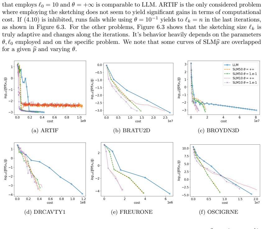
- The adaptive rule that shrinks $\ell_k$ only when $\theta_k^*\le\theta$ prevents the step from being too poor an approximation of the full Gauss-Newton model; the numerical experiments show that this check, with a moderate threshold such as $\theta=10^{-1}$, avoids the stagnation seen when $\theta=\infty$.
- Under the local error-bound assumptions, every string of $\bar k$ consecutive true iterations retains the deterministic local contraction rates (linear for $\beta=0$, and with the superlinear/quadratic exponent $(1+\beta)^{\bar k}$ for $\beta\in(0,1]$), with probability at least $(1-\pi_M)^{\bar k}$, so local fast convergence is not destroyed by sketching when the embeddings hold.
Reading between the lines
- The proof template, uniform decrease at true iterations plus a martingale count of true iterations, does not use the specific Levenberg-Marquardt form in a tight way, so the same variable-dimension strategy and $\theta$-style quality check should transfer to randomized trust-region or cubic-regularization methods for nonlinear least squares; testing this transfer is a natural next step.
- The adaptive $\ell_k$ appears to act as an online estimate of the local rank of $J(x_k)$: the experiments that record $\ell_k$ along the iterations show it changing in response to step quality, and a direct experiment comparing $\ell_k$ with rank$(J(x_k))$ would make this precise.
- When the full gradient can be evaluated, the $\theta_k^*$ check costs $O(mn)$ per iteration, which may dominate the savings when $n$ is very large; replacing $\theta_k^*$ by an estimate from a second independent sketch would extend the method to regimes where forming $J^T F$ and $J^T J s$ is the bottleneck.
Editorial analysis
A structured set of objections, weighed in public.
Referee Report
Summary. The paper proposes a stochastic inexact Gauss-Newton / Levenberg-Marquardt method for nonlinear least-squares in which each trial step is computed in a random subspace of variable dimension. The subspace size is adapted using the Armijo condition and, in a revised strategy, a check on the accuracy of the step relative to the full Gauss-Newton model. The main theoretical claims are a high-probability global iteration-complexity bound of order O(τ^-2) for driving the gradient norm below τ, and a local convergence analysis showing linear, superlinear, or quadratic decrease of the distance to the stationary set under an error-bound condition, with probability (1-π_M)^k for k consecutive true iterations. Numerical experiments on CUTEst problems and binary classification datasets compare the adaptive sketching method against deterministic Levenberg-Marquardt and fixed-size sketching variants.
Significance. If the global complexity theorem were fully established, the paper would provide a useful extension of randomized subspace methods to variable-dimension Levenberg-Marquardt methods, preserving the deterministic worst-case iteration complexity while reducing the per-iteration linear-algebra cost. The local analysis (Lemmas 5.7-5.12 and Theorem 5.13) is detailed, internally consistent, and appears to be a genuine contribution, and the numerical study is broad and carefully reported, including comparisons with constant-size sketching. However, the advertised global complexity result is not proven as written because of a gap between true iterations and successful iterations, so the main theoretical selling point currently rests on an unproved step.
major comments (2)
- [Section 3, Lemma 3.8(ii) and Theorem 3.10] The proof of the global complexity bound conflates the event 'iteration is true' with the event 'iteration is successful.' In Lemma 3.8(ii), N_S is defined as N_S = Σ_{k=0}^{N-1} T_k, where T_k is the true-iteration indicator from Definition 3.2 and Assumption 3.6, but the lemma calls this 'the number of successful iterations.' Lemma 3.5(i), which is the only source of the uniform decrease h(τ,t_k), applies only to iterations that are both true and successful. Lemma 3.3 only guarantees success when t_k < t_low, and Step 2 of Algorithm 2.1 sets t_{k+1} = min{t_max, γ^{-1} t_k} after a success, so t_k can repeatedly return above t_low; true-but-unsuccessful iterations are not confined to a finite transient. A Chernoff-type lower bound on the count of true iterations therefore cannot be inserted into the decrease-summing argument of [13, Theorem 2.1] unless one also controls the gap between true and successful iterations. Consequently, Eq. (3.10) and the probability bound P(N ≥ N_τ) ≥ 1 - exp(-δ_1^2(1-δ_M)N/2) are not established as written.
- [Section 3, Assumption 3.4 and Lemma 3.5(i)] Assumption 3.4 is load-bearing for the global complexity result because it turns the Armijo decrease into the uniform lower bound h(τ,t_k) in Lemma 3.5(i), but the paper does not show when this assumption is available. The ε-subspace embedding property (4.2) only gives σ_1(M_k J(x_k)^T) ≤ (1+ε)^{1/2} σ_1(J(x_k)^T), as proved in Theorem 4.3(ii), so a k-independent constant σ^† requires a uniform bound on ||J(x_k)|| along the generated sequence. The paper neither proves such a bound nor states it as a separate global hypothesis. Since the algorithm allows the iterates to move freely in R^n, this is a real restriction on the applicability of Theorem 3.10 and should be stated explicitly or derived from additional assumptions on the problem.
minor comments (4)
- [Lemma 3.9] The definition of ψ_t appears to contain a typo: as written, ψ_t = min{1, log_γ(t_low/t_0)} can be negative or non-integer when t_0 < t_low, and the stated inequality t_min ≤ min{t_low, γ t_0} does not follow without correction. Please revise the formula or clarify the intended floor/ceiling operations.
- [Section 3 and Appendix A.2] The proof of Lemma 3.8(ii) is deferred entirely to '[13, Proof of Lemma A.1]', but Lemma 3.8 is a central ingredient with a redefined counting variable; the authors should provide a self-contained proof or explicitly verify that the cited argument still applies to their definition of T_k.
- [Section 6.1] There are several small presentation issues: 'It's behavior' should be 'Its behavior'; 'SLMbpthe' should be 'SLMbp the'; and the caption of Table 6.3 mentions 'LLM and SLM50' while the table appears to report only SLM50 data.
- [Algorithm 4.1 and Section 4] The use of the symbol θ both for the threshold in (4.10) and for the accuracy measure θ_k^* in (4.1) is potentially confusing; a different symbol for the threshold, or an explicit statement that the meanings are distinct, would improve readability.
Circularity Check
No significant circularity: the complexity and local-convergence results are derived from explicit independent assumptions, with external prior work carrying the probabilistic machinery.
full rationale
The manuscript does not exhibit a circular derivation. Theorem 3.10's probabilistic iteration bound is obtained by combining explicit Assumptions 3.1, 3.4, and 3.6 with Lemma 3.5 (the Armijo decrease), Lemma 3.8 (the lower tail for true iterations), and Lemma 3.9 (the minimum step length). Lemma 3.8 and Lemma 3.9 explicitly invoke [13] (Cartis et al.) and Lemma 3.7 follows Shao's thesis [30]; these are external sources, not the authors' own prior work. The only self-references, [3] and tangentially [19], are contextual or are used in parallel with [1] for the local analysis; they do not supply the load-bearing embedding or complexity facts. No parameter is fitted to observations that are later 'predicted', and the variable-size update (Algorithm 4.1) is tested only numerically. The weakest point, Assumption 3.4, is an explicit regularity assumption rather than a restatement of the target result; whether it holds for a given sequence is a correctness and assumption-checking question, not an input-output equivalence. Similarly, the concern that Lemma 3.8's N_S is defined as the sum of true-iteration indicators T_k while Lemma 3.5's decrease applies to true-and-successful iterations is a potential proof gap, but it is not circularity: it does not make the theorem's conclusion equal to its assumptions by construction. Hence no step in the claimed derivation chain reduces to its own input.
Assumptions & free parameters
free parameters (5)
- theta (threshold in (4.10)) =
infinity, 1e-1, 1e-3 in experiments
- ell_0 (initial sketching size) =
10% or 50% of n
- eta (forcing term) =
0 or 1e-3
- mu_k (regularization) =
1e-4
- c, gamma, gamma_hat, t_max, ell_min, ell_max =
c=1e-4, gamma=0.5, gamma_hat=0.909, t_max=1, ell_min=n/10, ell_max=n
assumptions (8)
- domain assumption Assumption 3.1: f is continuously differentiable, bounded below, and grad f is L-Lipschitz.
- domain assumption Assumption 3.4: sigma_1(M_k J(x_k)^T J(x_k) M_k^T) <= sigma_dagger for all true iterations.
- domain assumption Assumption 3.6: true iterations occur with probability at least 1-delta_M conditional on the past, with conditional independence.
- domain assumption Assumption 5.2: rank(J^T J) is constant r and its smallest nonzero eigenvalue is at least lambda_min on B_zeta.
- domain assumption Assumption 5.3: omega dist(x, Omega*) <= ||grad f(x)|| (error bound).
- domain assumption Assumption 5.4: ||J(x)^T F(z)|| <= sigma ||x-z||^{1+beta} for z in B_zeta ∩ Omega* (residual growth).
- domain assumption Assumption 5.6: embedding events bT_k occur with probability at least 1-pi_M conditional on the past.
- domain assumption Assumption 5.9: specific choices of eta_k and mu_k proportional to ||J^T F||^beta, and sigma < xi omega/(2+c_1) when beta=0.
Cite this review
Pith. "Pith review of A variable dimension sketching strategy for nonlinear least-squares." pith.science (2026). https://pith.science/paper/XSZ2S2SG
@misc{pith2026250603965,
  author       = {Pith},
  title        = {Pith review of: A variable dimension sketching strategy for nonlinear least-squares},
  year         = {2026},
  howpublished = {\url{https://pith.science/paper/XSZ2S2SG}},
  note         = {Machine review of arXiv:2506.03965}
}
read the original abstract
We present a stochastic inexact Gauss-Newton method for the solution of nonlinear least-squares. To reduce the computational cost with respect to the classical method, at each iteration the proposed algorithm approximately minimizes the local model on a random subspace. The dimension of the subspace varies along the iterations, and two strategies are considered for its update: the first is based solely on the Armijo condition, the latter is based on information from the true Gauss-Newton model. Under suitable assumptions on the objective function and the random subspace, we prove a probabilistic bound on the number of iterations needed to drive the norm of the gradient below any given threshold. Moreover, we provide a theoretical analysis of the local behavior of the method. The numerical experiments demonstrate the effectiveness of the proposed method.
Figures


Figures from the paper (7 more)


Reference graph
Works this paper leans on
-
[1]
Behling, R., Goncalves, D.S., Santos, S.A.,Local Convergence Analysis of the Levenberg-Marquardt Frame- work for Nonzero-Residue Nonlinear Least-Squares Problems Under an Error Bound Condition, Journal of Optimization Theory and Applications, 183, pp. 1099–1122, 2019
work page 2019
-
[2]
S. Bellavia, G. Gurioli, B. Morini, P. L. Toint,Trust-region algorithms: probabilistic complexity and intrinsic noise with applications to subsampling techniques, EURO Journal on Computational Optimization, 10, pp. 1–37, 2022
work page 2022
-
[3]
S. Bellavia, G. Malaspina, B. Morini,Inexact Gauss-Newton methods with matrix approxima- tion by sampling for nonlinear least-squares and systems, Mathematics of Computation, DOI: https://doi.org/10.1090/mcom/4073, 2025
-
[4]
S. Bellavia, N. Kreji´ c, B. Morini, S. Rebegoldi,A stochastic first-order trust-region method with inexact restoration for finite-sum minimization, Computational Optimization and Applications, 84, pp. 53-84 2023
work page 2023
-
[5]
S. Bellavia, B. Morini,Strong local convergence properties of adaptive regularized methods for nonlinear least squares, IMA Journal of Numerical Analysis, 35, pp. 947-968, 2015
work page 2015
-
[6]
A.S. Berahas, L. Cao, K. Scheinberg,Global convergence rate analysis of a generic line search algorithm with noise, SIAM Journal on Optimization, 31, pp. 1079–1603, 2021
work page 2021
-
[7]
A. Bjork, Numerical Methods for Least Squares Problems, Society for Industrial and Applied Mathematics, 1996
work page 1996
-
[8]
I. Bongartz, A. R. Conn, N. I. M. Gould, and Ph. L. Toint.CUTE: Constrained and Unconstrained Testing Environment.ACM Transactions on Mathematical Software, 21(1), pp. 123–160, 1995
work page 1995
Show all 33 references
-
[9]
Blanchet, C
J. Blanchet, C. Cartis, M. Menickelly, K. Scheinberg,Convergence Rate Analysis of a Stochastic Trust Region Method via Submartingales, INFORMS Journal on Optimization, 1, pp. 92-119, 2019
2019
-
[10]
Byrd , G.M
R.H. Byrd , G.M. Chin, W. Neveitt, J. Nocedal,On the Use of Stochastic Hessian Information in Opti- mization Methods for Machine Learning, SIAM Journal on Optimization, 21(3), pp. 977-995, 2011
2011
-
[11]
Byrd, G.M
R.H. Byrd, G.M. Chin, J. Nocedal, Y. WuSample size selection in optimization methods for machine learning, Mathematical Programming, 134(1), pp. 127-155, 2012
2012
-
[12]
Byrd, S.L
R.H. Byrd, S.L. Hansen, J. Nocedal, Y. Singer,A Stochastic Quasi-Newton Method for Large-Scale Opti- mization, SIAM Journal on Optimization, 26(2), pp. 1008–1021, 2016
2016
-
[13]
Cartis, J
C. Cartis, J. Fowkes, Z. Shao,Randomised Subspace Methods for Non-Convex Optimization, with Applica- tions to Nonlinear Least-Squares, 2022, arXiv:2211.09873v1
2022 arXiv
-
[14]
Cartis, J
C. Cartis, J. Fowkes, Z. Shao,A Randomised Subspace Gauss-Newton Method for Nonlinear Least-Squares, 2022, arXiv:2211.05727v1
2022 arXiv
-
[15]
Cartis, Z
C. Cartis, Z. Shao, E. Tansley,Random Subspace Cubic-Regularization Methods with applications to Low- Rank Functions, 2024, arXiv:2501.09734v1
2024 arXiv
-
[16]
Cartis, K
C. Cartis, K. Scheinberg,Global convergence rate analysis of unconstrained optimization methods based on probabilistic model, Mathematical Programming, 169, pp. 337–375, 2017
2017
-
[17]
R. Chen, M. Menickelly, K. Scheinberg,Stochastic optimization using a trust-region method and random models, Mathematical Programming, 169, pp. 447-487, 2018
2018
-
[18]
Dennis, R.B
J.E. Dennis, R.B. Schnabel,Numerical methods for unconstrained optimization and nonlinear equations, Prentice Hall, Englewood Cliffs, NJ, 1983
1983
-
[19]
Fodor, D
L. Fodor, D. Jakoveti´ c, N. Kreji´ c, G. Malaspina,Parallel Inexact Levenberg-Marquardt Method for Nearly- Separable Nonlinear Least Squares, arXiv preprint arXiv:2312.09064, 2023
2023 arXiv
-
[20]
D. C.-L. Fong, M. A. Saunders,LSMR: An iterative algorithm for sparse least-squares problems, SIAM J. Sci. Comput. 33:5, 2950-2971, 2011 29
2011
-
[21]
N. I. M. Gould, D. Orban, and Ph. L. Toint.CUTEst: a constrained and unconstrained testing environ- ment with safe threads for mathematical optimization. Computational Optimization and Applications, 60(3):545-557, 2015
2015
-
[22]
B. Jin, K. Scheinberg, M. Xie,High Probability Complexity Bounds for Adaptive Step Search Based on Stochastic Oracles, SIAM Journal on Optimization, 34(3), pp. 2169–3166, 2024
2024
-
[23]
Guyon, S
I. Guyon, S. Gunn, A. Ben-Hur, G. Dror, Gisette [Dataset], UCI Machine Learning Repository, 2004
2004
-
[24]
M. W. Mahoney,Randomized Algorithms for Matrices and Data, Fund. Trends Mach. Learn., 3(2), pp. 123–224, 2011
2011
-
[25]
Martinsson, J
P.G. Martinsson, J. A. Tropp,Randomized numerical linear algebra: Foundations and algorithms, Acta Numerica, 29, pp. 403–572, 2020
2020
-
[26]
Pang,Error bounds in mathematical programming Mathematical Programming, 79, pp
J.S. Pang,Error bounds in mathematical programming Mathematical Programming, 79, pp. 299-332, 1997
1997
-
[27]
Paquette, K
C. Paquette, K. Scheinberg,A Stochastic Line Search Method with Expected Complexity Analysis, SIAM Journal of Optimization, 30, pp. 349–376, 2020
2020
-
[28]
Pilanci, M.J
M. Pilanci, M.J. Wainwright,Newton sketch: A near linear-time optimization algorithm with linear- quadratic convergence, SIAM Journal on Optimization 27(1), pp. 205–245, 2017
2017
-
[29]
Pinheiro, S
R. Pinheiro, S. M. L. de Lima, S. Murilo, E. Albuquerque, D. Souza, T. Monteiro, P. Lopes, R. Lima, J. Oliveira, S. Silva, REJAF ADA [Dataset], UCI Machine Learning Repository, 2019
2019
-
[30]
Shao,On Random Embeddings and Their Application to Optimization, PhD thesis, University of Oxford, Oxford, UK, 2021
Z. Shao,On Random Embeddings and Their Application to Optimization, PhD thesis, University of Oxford, Oxford, UK, 2021
2021
-
[31]
Tropp,An Introduction to Matrix Concentration Inequalities, Foundations and Trends in Machine Learning, 8, pp
J.A. Tropp,An Introduction to Matrix Concentration Inequalities, Foundations and Trends in Machine Learning, 8, pp. 1–230, 2015
2015
-
[32]
R. Yuan, A. Lazaric, R. M. Gower,Sketched Newton–Raphson, SIAM Journal on Optimization, 32, pp. 1499-2459, 2022
2022
-
[33]
D. P. Woodruff,Sketching as a tool for numerical linear algebra, Foundations and Trends in Theoretical Computer Science, 10, No. 1-2, pp. 1–157, 2014 30
2014
Reviewed August 7, 2026 · model on record in the stance chip above.
Discussion (0). Sign in to comment.