Estimating properties of a homogeneous bounded soil using machine learning models

Konstantinos Kalimeris; Leonidas Mindrinos; Nikolaos Pallikarakis

REVIEW 3 major objections 6 minor 26 references

Estimating properties of a homogeneous bounded soil using machine learning models

T0 review · 3 major / 6 minor · reviewed 2026-08-07 · deepseek-v4-flash

Challenge this review Re-run · record.json Download PDF Read on arXiv ↗

Pith's one-line read This paper claims that support vector machines and neural networks recover soil diffusivity and hydraulic conductivity from moisture time series with near-perfect accuracy, outperforming tree-based and instance-based regressors.

desk verdict Solid synthetic ML benchmark with a careful pipeline; the near-perfect R2 reflects the smooth Fokas forward map, not field skill, and the title overclaims. read the letter →

arxiv 2506.04256 v1 pith:EX72M6J7 submitted 2025-06-02 physics.geo-ph cs.LG

Konstantinos Kalimeris , Leonidas Mindrinos , Nikolaos Pallikarakis This is my paper

classification physics.geo-phcs.LG MSC 35G1635R3076S0586-10

keywords verticalinfiltrationinverseproblemsoilhydraulicpropertiesmachinelearningmulti-outputregressionFokasmethodsupportvectorneuralnetworks

verification ladder T0 review T1 audit T2 compute T3 formal

The pith

A machine-rendered reading of the paper's core claim, the machinery that carries it, and where it could break.

The reading

The paper asks whether machine learning can recover two soil properties, water diffusivity $D$ and hydraulic conductivity $K$, from time series of water-content readings at three depths in a homogeneous, bounded soil under flooding. It generates training data by numerically evaluating an exact integral solution of the governing linear infiltration PDE, obtained with the Fokas method, for many random pairs $(K,D)$, and it adds Gaussian noise to the test sets to mimic imperfect measurements. Five regression models are compared under full, noisy, and limited data. The central claim is that support vector machines (SVM) and neural networks (NN) consistently outperform random forests, XGBoost, and $k$-nearest neighbors, reaching $R^2$ scores of 1.0000 for $D$ and effectively 1.0000 for $K$ on exact data while degrading least under noise, feature reduction, and smaller training sets. A sympathetic reader would care because the result points toward fast, purely data-driven estimation of soil parameters that could complement slower laboratory or iterative inversion methods, at least in controlled homogeneous settings.

What carries the argument

The load-bearing object is the integral representation (2), the Fokas-method solution of the advection-diffusion initial-boundary value problem (1) for water content $\theta(x,t)$; this is what turns a pair $(K,D)$ into a 30-dimensional vector of moisture values at depths $L/4$, $L/2$, $3L/4$ and ten time steps. The machine learning models then learn the inverse map from those moisture vectors back to $(K,D)$. The Fokas construction matters because it evaluates the direct problem cheaply for thousands of parameter pairs, which is what makes the supervised training set possible.

What would settle it

Run a controlled laboratory column of length $L=140$ cm with independently measured $K$ and $D$, record moisture at $x=L/4, L/2, 3L/4$ at the same ten time steps, and apply the trained SVM and NN regressors: if their $R^2$ on these real measurements drops substantially below the reported values, or if their errors are comparable to those of iterative inverse solvers, the transferability claim is false.

Watch

Extended reading notes

Core claim

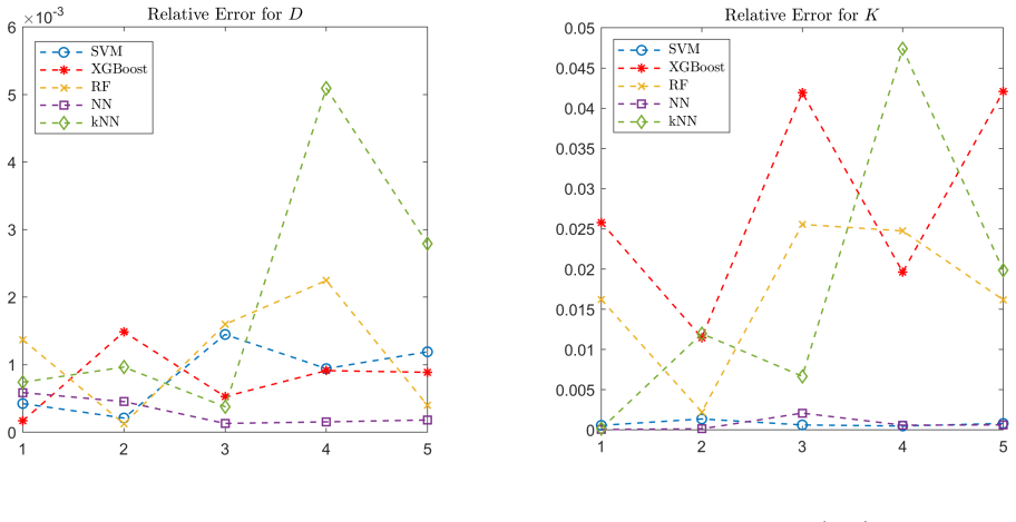
On the paper's own terms, the discovery is that the inverse map from moisture measurements to soil parameters is learnable with near-perfect fidelity: on the full exact dataset both SVM and NN achieve $R^2 = 1.0000$ for $D$ and effectively perfect scores for $K$ (SVM 1.0000, NN 0.9999), with NN reaching the smallest errors for $D$ (MSE 0.5293, MAE 0.5640 in the paper's units) and SVM reaching essentially zero error for $K$ (MAE 0.0042). The paper further claims that $D$ is systematically easier to predict than $K$; that 2% and 5% Gaussian noise in the test set inflates errors for all models but leaves SVM and NN as the most stable, while XGBoost collapses for $K$ ($R^2$ down to 0.5541 at 2% noise); and that reducing the dataset from 2000 to 500 samples, or from 30 features to the five most important ones, barely hurts SVM and NN. Feature analysis singles out moisture measured at $x=L/4$ at late times as the most informative input across models.

Load-bearing premise

The simulated moisture data, generated by numerically evaluating the Fokas-method solution of a linear infiltration equation with constant $K$ and $D$, are assumed to represent real water-content measurements in a homogeneous bounded soil well enough that near-perfect test accuracy carries over to the field; the paper itself notes synthetic data cannot capture full field complexity and heterogeneity.

Editorial extensions

If this is right

If the claim holds, field estimation of $D$ and $K$ becomes a one-shot regression call from roughly ten to thirty moisture readings, with no iterative PDE solver needed at prediction time.
Sensor campaigns can be shortened: measurements near the surface at early-to-mid times carry most of the signal, so a single probe around $x=L/4$ sampled hourly may suffice for $D$.
Applications should treat $K$ as the harder target: with noise or limited data, conductivity predictions carry substantially more uncertainty than diffusivity predictions.
A 500-sample synthetic training set is enough for near-optimal SVM and NN performance, lowering the data-generation cost for similar inverse problems.
Tree-based models (XGBoost, random forest) are not the right default for this problem, since they degrade sharply under input noise.

Reading between the lines

Editorial extensions of the paper, not claims the author makes directly.

The near-perfect scores probably reflect the smoothness of the map from synthetic moisture features to $(K,D)$ in a constant-coefficient linear PDE; real heterogeneous field soils add variability that these numbers do not bound, so field accuracy may be much lower.
The same Fokas-based data generator could be used to pre-train models that are later fine-tuned on a small set of field measurements, a hybrid strategy the paper leaves implicit.
The top-ranked feature $\Theta_{1,10}$ suggests a concrete experiment: train the models with that single sensor deleted and measure how much accuracy drops, which would test whether one depth-time pair really carries most of the information.
At 5% noise the ranking shifts, with $k$NN becoming comparable to SVM for $K$; this suggests model choice may depend on the expected noise regime and should be re-examined on real data.

Share X Bluesky LinkedIn Reddit HN

Editorial analysis

A structured set of objections, weighed in public.

Desk editor's note, referee report, and a circularity audit.

Desk Editor's Note

read the letter

Quick read: this is a competent, clearly written benchmark comparison of five ML regressors on synthetic data for estimating constant conductivity K and diffusivity D in a homogeneous soil column. The data are generated by numerically evaluating the authors' own Fokas-method solution to the linear advection-diffusion IBVP. What the paper does well: the ML pipeline is careful—80/10/10 split, scaling fit only on training, 5-fold CV, noise added only to test, and a sensible feature-importance analysis. The internal ranking (SVM and NN best, XGBoost in the middle, RF and kNN weakest) is honestly reported and supported by the tables. The introduction also contains an accurate disclaimer that synthetic data cannot capture field heterogeneity, so the authors are aware of the limitation.

The soft spots are in the framing, not the execution. The title and abstract say 'estimating properties of a homogeneous bounded soil using ML models' and call SVM/NN 'the most reliable models for this inverse modeling task.' Given that all test data come from the same deterministic forward model, near-perfect R2 is exactly what you would expect: the map from 30 moisture readings to (K,D) is smooth and well-posed within a narrow parametric family (K in [3,6], D in [1080,2160]). That is a valid synthetic benchmark, but it does not support a conclusion about real soil-property estimation. The authors concede this in Section 1, yet the opacity in title/abstract is a real overreach. Also, no code or data are provided, and the test-set MSE/MAE come from a single random split with no confidence intervals; the 5-fold CV is only reported as R2 means. Minor issues: unit inconsistency for D (cm^2/sec vs cm^2/h), several typos ('seams,' 'oven thousand'), and at least one suspicious relative-change number (kNN R2 +73.3% in Table 13—probably a misplaced decimal or an off-by-a-hundred error).

None of this sinks the paper. As an internal comparison of ML models on a user-friendly synthetic dataset, it is useful. The Fokas-solution data generator is a nice resource, and the feature importance results could inform sensor placement. The right fix is to reframe claims to 'on this simulated dataset,' add reproducibility (code/data), and report error bars or repeated splits. Who is this for: researchers in ML-based inverse problems who want a baseline for soil parameter regression, and anyone looking for a fast synthetic-data generator. It deserves peer review, not desk rejection, but a serious referee should push on the generalization claims and request the code.

Referee Report

3 major / 6 minor

Summary. The paper addresses the inverse problem of estimating hydraulic conductivity K and water diffusivity D from water-content observations in a homogeneous bounded soil. Training and test data are generated synthetically by numerically evaluating the Fokas-method integral solution (Eq. 2) for randomly drawn (K, D) pairs. Five machine learning regressors (SVM, XGBoost, Random Forest, Neural Network, kNN) are compared under full, noisy, and limited data conditions, together with feature-importance analysis and PCA/UMAP dimensionality reduction. The reported results show SVM and NN achieving near-perfect R^2 and the lowest errors for both target parameters, and the conclusions identify these two models as the most reliable for the inverse modeling task.

Significance. If the central claim were established for real soils, the paper would provide a useful practical recipe for sensor placement and model choice in soil-property estimation. The manuscript has genuine strengths: preprocessing is carefully separated so that scaling parameters are learned only from the training set; 5-fold cross-validation is used for model selection; noise is added only to the test set to probe generalization; and the feature-importance analysis gives actionable insight into which measurement locations and times matter most. However, the entire benchmark is closed-loop: all data come from the authors' own Fokas-method forward model with constant K and D, and the paper itself acknowledges in Section 1 that synthetic data cannot capture the full complexity of field conditions. The near-perfect accuracies reported in Tables 6-7 may therefore reflect interpolation within a smooth parametric family rather than a transferable skill for real field data.

major comments (3)

[Section 1, Section 4.1, Conclusions] The central claim that SVM and NN are 'the most reliable models for this inverse modeling task' is not established for actual soil-property estimation. Both training and test data are produced by numerically evaluating the same Fokas-method solution (Eq. 2), with constant K and D and simplified boundary conditions, and the paper explicitly concedes in Section 1 that simulated data fail to capture the full complexity and heterogeneity of field conditions. The near-perfect R^2 scores in Tables 6-7 may reflect the smoothness and low effective dimensionality of the map from 30 moisture measurements to (K, D) within this parametric family, not robustness to real-world conditions. Please either validate the models on independent field or laboratory data, or restrict the abstract and conclusion claims explicitly to the synthetic benchmark and present the study as a controlled methodological comparison.
[Section 4.1, Tables 6-7 and 10-11] All point estimates of MSE and MAE are based on a single 10% test split, and no confidence intervals or repeated random splits are provided. The cross-validation results in Tables 10-11 report standard deviations of 0.0000 for several models, which appears to be an artifact of rounding rather than a meaningful zero variability. Please report uncertainty estimates from repeated train/test splits or bootstrap resampling, and give the cross-validation standard deviations with enough significant digits to be interpretable. Without this, the claim that SVM and NN 'consistently' outperform the other models is not statistically supported.
[Section 4.4, Eq. (4)] The noise study adds Gaussian noise only to the test set, while the models are trained on exact, noise-free data, as stated in Section 2.1. This design tests robustness to unseen distortions but does not reproduce realistic conditions in which calibration errors and sensor noise also contaminate training data. The conclusion that SVM and NN are the 'most stable' models under noise should be tempered, or the experiments should be supplemented with a condition in which noise is also added to the training set (e.g., noise augmentation). The current design cannot distinguish between a model that is intrinsically robust to noise and one that simply benefits from being trained on a noise-free idealization of the same forward model.

minor comments (6)

[Section 2.1] The diffusivity D is first generated in cm^2/sec and then reported in cm^2/h (1080-2160 cm^2/h). State the conversion factor explicitly in the text to avoid unit confusion.
[Table 7] The SVM row for K reports MSE = 0.0000 while MAE = 0.0042; reporting more significant digits would make the metrics internally consistent and more informative.
[Section 4.4, Tables 17 and 19] Relative change percentages computed against zero or near-zero baselines (e.g., '+∞%' for SVM in Table 17) are not meaningful; report the absolute error values alongside the relative changes.
[Section 4.4] There are typos in the text: 'oven thousand' should be 'over thousand' and 'seams' should be 'seems'.
[Section 3.2 and Section 4.3.3] The hyperparameter grid for GridSearchCV and the UMAP settings (e.g., n_neighbors, min_dist, metric) are not reported, which limits reproducibility. Please include these details.
[Tables 10 and 11] The standard deviation values of 0.0000 for several models are likely due to rounding to four decimal places; reporting additional decimal places would clarify whether the cross-validation variability is truly negligible.

Circularity Check

0 steps flagged · score 0.0 of 10

No significant circularity: the ML inverse mapping is learned from generic supervised training, not derived from the forward equations; the self-cited Fokas solution is independent support, and the synthetic-data limitation is an external-validity caveat, not a circular reduction.

full rationale

The derivation chain is not circular. The soil-moisture data are generated by numerically evaluating the Fokas-method solution (2) of the linear IBVP (1), with K and D drawn randomly from stated ranges. This forward map is the input generator, not a fitted parameter of any ML model. The ML models are trained on (feature, label) pairs produced by this generator under a standard 80/10/10 split with 5-fold cross-validation, and hyperparameters are selected by grid search on validation data only. No test label is used to fit the models or to post-select the reported metrics. The predicted outputs K and D are not defined in terms of the input moisture features; they are learned generic regressions, so the near-perfect R2 values in Tables 6-7 are empirical fits to a smooth deterministic family, not quantities forced by construction from the inputs. The self-citation [2] supplies the forward solution, but that solution is a parameter-free analytical result for the stated PDE with stated boundary and initial data, and the paper notes it has been validated against established approximate analytical solutions; it does not assume the ML ranking or the inverse mapping. The acknowledged limitation that synthetic data "fail to capture the full complexity and heterogeneity of field conditions" (Section 1) is an external-validity caveat, not a circular reduction. The closed synthetic-data loop means the benchmark measures inversion skill within the Fokas-generated family, but no equation is equivalent to its own input and no fitted parameter is renamed as a prediction. Thus no significant circularity; score 0.

Assumptions & free parameters 14 free parameters · 4 assumptions · 0 invented entities

The central claim rests on the fidelity of the synthetic data generation, which uses the authors' own forward solution and chosen parameter ranges. The ML hyperparameters are tuned to the data but are standard practice. No new physical entities are introduced.

free parameters (14)

SVR regularization c = 1000
Chosen via grid search to minimize validation MSE; affects model complexity.
SVR kernel coefficient gamma = 0.01
Chosen via grid search; controls RBF kernel influence.
SVR epsilon = 0.01
Insensitivity tube width, tuned by grid search.
NN hidden layer sizes = [128, 64, 32]
Architecture chosen by the authors, not derived from theory.
NN L2 regularization = 2e-4
Weight decay parameter.
NN learning rate = 0.0001
Adam optimizer learning rate.
XGBoost max_depth = 7
Tuned via grid search.
XGBoost learning_rate = 0.2
Tuned via grid search.
XGBoost number of estimators = 300
Tuned via grid search.
RF max_depth = 20
Tuned via grid search.
kNN number of neighbors = 3
Tuned via grid search.
Data generation K range = [3, 6] cm/h
Chosen by hand, representative of some soils.
Data generation D range = [1080, 2160] cm2/h
Chosen by hand, representative.
Noise levels = 2%, 5%
Chosen to simulate measurement error.

assumptions (4)

domain assumption The integral representation (2), derived via the Fokas method in [2], gives the correct solution to the IBVP (1).
All synthetic data are generated from this solution; if it is wrong, every training/test feature is invalid. The paper does not re-derive it.
domain assumption The linear advection-diffusion PDE (1) with constant K and D is an adequate model for vertical infiltration in a homogeneous bounded soil under flooding.
The entire inverse problem is built on this physical model; real soils are heterogeneous and nonlinear, so this is a simplifying assumption.
domain assumption The boundary and initial conditions (theta0=0.03, theta1=0.3 cm3/cm3) and the parameter ranges K in [3,6] cm/h and D in [1080,2160] cm2/h are representative of field conditions.
These values are taken from the literature or chosen by the authors; they affect the domain of the learned mapping.
domain assumption Gaussian noise with sigma = delta * sigma_Theta models realistic measurement error in soil moisture sensors.
The noise model (4) is an assumption about sensor errors; if real errors are non-Gaussian or heteroscedastic, the noise-robustness results may not transfer.

how reviews work

0 comments

Cite this review

Pith. "Pith review of Estimating properties of a homogeneous bounded soil using machine learning models." pith.science (2026). https://pith.science/paper/EX72M6J7

@misc{pith2026250604256,
  author       = {Pith},
  title        = {Pith review of: Estimating properties of a homogeneous bounded soil using machine learning models},
  year         = {2026},
  howpublished = {\url{https://pith.science/paper/EX72M6J7}},
  note         = {Machine review of arXiv:2506.04256}
}

abstract

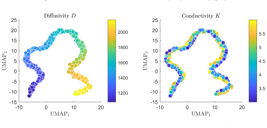
This work focuses on estimating soil properties from water moisture measurements. We consider simulated data generated by solving the initial-boundary value problem governing vertical infiltration in a homogeneous, bounded soil profile, with the usage of the Fokas method. To address the parameter identification problem, which is formulated as a two-output regression task, we explore various machine learning models. The performance of each model is assessed under different data conditions: full, noisy, and limited. Overall, the prediction of diffusivity $D$ tends to be more accurate than that of hydraulic conductivity $K.$ Among the models considered, Support Vector Machines (SVMs) and Neural Networks (NNs) demonstrate the highest robustness, achieving near-perfect accuracy and minimal errors.

Figures

Figures reproduced from arXiv: 2506.04256 by the authors.

**Figure 1.** Moisture profiles θ in soil for different infiltration times due to flooding (left). Moisture profiles at given depth positions with respect to time (right). noise magnitude is proportional to the variability of the data. Noise is introduced exclusively in the test set, ensuring that the model is trained solely on exact (noise-free) data and is exposed to noisy inputs only during evaluation. This setup poses a great… view at source ↗

**Figure 2.** PCA dimension reduction for D (left) and K (right) [PITH_FULL_IMAGE:figures/full_fig_p012_2.png] view at source ↗

**Figure 3.** UMAP dimension reduction for D (left) and K (right). upper region of the PC1–PC2 plane, while in UMAP space, K is more diffusely distributed, suggesting a more complex and nonlinear dependency on the input features. As we illustrate in the following, this increased complexity contributes to the relatively lower accuracy observed when predicting K, particularly under noisy conditions, an outcome consistent with the … view at source ↗

Figures from the paper (12 more)

**Figure 4.** Figure 4: Relative errors between the actual and predicted values of [PITH_FULL_IMAGE:figures/full_fig_p015_4.png]

**Figure 5.** Figure 5: The loss function of the neural network model for exact data. [PITH_FULL_IMAGE:figures/full_fig_p016_5.png]

**Figure 6.** Figure 6: Regression plots of D [cm2/h] (left) and K [cm/h] (right) in the test set for exact data. 26 [PITH_FULL_IMAGE:figures/full_fig_p026_6.png]

**Figure 7.** Figure 7: Residual plots of D [cm2/h] (left) and K [cm/h] (right) in the test set for exact data. 27 [PITH_FULL_IMAGE:figures/full_fig_p027_7.png]

**Figure 8.** Figure 8: The five most important features identified for each model. [PITH_FULL_IMAGE:figures/full_fig_p028_8.png]

**Figure 9.** Figure 9: Regression plots of D [cm2/h] (left) and K [cm/h] (right) in the test set for data with 2% noise. Methods that achieved an R2 score greater than 0.95 for both outputs are presented. 29 [PITH_FULL_IMAGE:figures/full_fig_p029_9.png]

**Figure 10.** Figure 10: The impact of test set noise on the performance metrics for predicting [PITH_FULL_IMAGE:figures/full_fig_p030_10.png]

**Figure 11.** Figure 11: The impact of test set noise on the performance metrics for predicting [PITH_FULL_IMAGE:figures/full_fig_p031_11.png]

**Figure 12.** Figure 12: The effect of dataset size on the metrics for predicting [PITH_FULL_IMAGE:figures/full_fig_p032_12.png]

**Figure 13.** Figure 13: The effect of dataset size on the metrics for predicting [PITH_FULL_IMAGE:figures/full_fig_p033_13.png]

**Figure 14.** Figure 14: The effect of feature count on the metrics for predicting [PITH_FULL_IMAGE:figures/full_fig_p034_14.png]

**Figure 15.** Figure 15: The effect of feature count on the metrics for predicting [PITH_FULL_IMAGE:figures/full_fig_p035_15.png]

Discussion (0). Sign in to comment.

Reference graph

Works this paper leans on

26 extracted references · 25 canonical work pages

[1]

Abbasi, J

F. Abbasi, J. Simunek, J. Feyen, M. T. Van Genuchten, and P. J. Shouse , Simultaneous inverse estimation of soil hydraulic and solute transport parameters from transient field experiments: Homogeneous soil , Transactions of the ASAE, 46 (2003), p. 1085

work page 2003
[2]

Argyrokastritis, K

I. Argyrokastritis, K. Kalimeris, and L. Mindrinos , An analytical solution for vertical infiltration in homogeneous bounded profiles , European Journal of Soil Science, 75 (2024), p. e13547

work page 2024
[3]

Chlouveraki, N

E. Chlouveraki, N. Katsenios, A. Efthimiadou, E. Lazarou, K. Kounani, E. Papakonstantinou, D. Vlachakis, A. Kasimati, I. Zafeiriou, B. Espejo-Garcia, and S. Fountas , Estimation of soil properties using hyperspectral imaging and machine learning , Smart Agricultural Technology, 10 (2025), p. 100790

work page 2025
[4]

F. A. Diaz-Gonzalez, J. Vuelvas, C. A. Correa, V. E. Vallejo, and D. Patino , Machine learning and remote sensing techniques applied to estimate soil indicators--review , Ecological Indicators, 135 (2022), p. 108517

work page 2022
[5]

A. S. Fokas , A unified transform method for solving linear and certain nonlinear pdes , Proceedings of the Royal Society of London. Series A: Mathematical, Physical and Engineering Sciences, 453 (1997), pp. 1411--1443

work page 1997
[6]

Forkuor, O

G. Forkuor, O. K. L. Hounkpatin, G. Welp, and M. Thiel , High resolution mapping of soil properties using remote sensing variables in south-western burkina faso: a comparison of machine learning and multiple linear regression models , PloS one, 12 (2017), p. e0170478

work page 2017
[7]

I. J. Goodfellow, Y. Bengio, and A. C. Courville , Deep Learning. Adaptive computation and machine learning , MIT Press, New York, 2016

work page 2016
[8]

Guellouz, B

L. Guellouz, B. Askri, J. Jaffr \'e , and R. Bouhlila , Estimation of the soil hydraulic properties from field data by solving an inverse problem , Scientific Reports, 10 (2020), p. 9359

work page 2020

Show all 26 references

[9]

Hastie, R

T. Hastie, R. Tibshirani, and J. Friedman , Elements of Statistical Learning: Data Mining, Inference and Prediction , Springer, New York, 2nd ed., 2001

2001
[10]

Heaton, S

J. Heaton, S. McElwee, J. Fraley, and J. Cannady , Early stabilizing feature importance for tensorflow deep neural networks , in 2017 International Joint Conference on Neural Networks (IJCNN), 2017, pp. 4618--4624

2017
[11]

I. T. Jolliffe , Principal Component Analysis , Springer, New York, 2002

2002
[12]

Kerkides, A

P. Kerkides, A. Poulovassilis, I. Argyrokastritis, and S. Elmaloglou , Comparative evaluation of analytic solutions in predicting soil moisture profiles in vertical one-dimensional infiltration under ponded and constant flux boundary conditions , Water Resources Management, 11...

1997
[13]

Khanal, J

S. Khanal, J. Fulton, A. Klopfenstein, N. Douridas, and S. Shearer , Integration of high resolution remotely sensed data and machine learning techniques for spatial prediction of soil properties and corn yield , Computers and electronics in agriculture, 153 (2018), pp. 213--225

2018
[14]

M. H. Kutner, C. J. Nachtsheim, J. Neter, and W. Li , Applied Linear Statistical Models , McGraw-Hill/Irwin, Boston, MA, 5th ed., 2005

2005
[15]

Le Bourgeois, C

O. Le Bourgeois, C. Bouvier, P. Brunet, and P.-A. Ayral , Inverse modeling of soil water content to estimate the hydraulic properties of a shallow soil and the associated weathered bedrock , Journal of Hydrology, 541 (2016), pp. 116--126

2016
[16]

McInnes, J

L. McInnes, J. Healy, and J. Melville , Umap: Uniform manifold approximation and projection for dimension reduction , arXiv preprint arXiv:1802.03426, (2018)

2018 arXiv
[17]

Moghadas and A

D. Moghadas and A. Badorreck , Machine learning to estimate soil moisture from geophysical measurements of electrical conductivity , Near Surface Geophysics, 17 (2019), pp. 181--195

2019
[18]

Padarian, B

J. Padarian, B. Minasny, and A. B. McBratney , Using deep learning to predict soil properties from regional spectral data , Geoderma Regional, 16 (2019), p. e00198

2019
[19]

Pallikarakis, A

N. Pallikarakis, A. Kalogeropoulos, and N. L. Tsitsas , Exploring the inverse line-source scattering problem in dielectric cylinders with deep neural networks , Physica Scripta, 99 (2024), p. 116013

2024
[20]

Pallikarakis and A

N. Pallikarakis and A. Ntargaras , Application of machine learning regression models to inverse eigenvalue problems , Comput. Math. Appl., 154 (2024), pp. 162--174

2024
[21]

W. J. Rawls, D. L. Brakensiek, and K. E. Saxtonn , Estimation of soil water properties , Transactions of the ASAE, 25 (1982), pp. 1316--1320

1982
[22]

Ritter, F

A. Ritter, F. Hupet, R. Mu \ n oz-Carpena, S. Lambot, and M. Vanclooster , Using inverse methods for estimating soil hydraulic properties from field data as an alternative to direct methods , Agricultural Water Management, 59 (2003), pp. 77--96

2003
[23]

B. C. Si and R. G. Kachanoski , Estimating soil hydraulic properties during constant flux infiltration inverse procedures , Soil Science Society of America Journal, 64 (2000), pp. 439--449

2000
[24]

Simunek and M

J. Simunek and M. T. Van Genuchten , Estimating unsaturated soil hydraulic properties from tension disc infiltrometer data by numerical inversion , Water Resources Research, 32 (1996), pp. 2683--2696

1996
[25]

B. B. Trangmar, R. S. Yost, and G. Uehara , Application of geostatistics to spatial studies of soil properties , Advances in agronomy, 38 (1986), pp. 45--94

1986
[26]

Zeraatpisheh, S

M. Zeraatpisheh, S. Ayoubi, A. Jafari, S. Tajik, and P. Finke , Digital mapping of soil properties using multiple machine learning in a semi-arid region, central iran , Geoderma, 338 (2019), pp. 445--452

2019

Pith tools

Reviewed August 7, 2026 · model on record in the stance chip above.

[1] [1]

Abbasi, J

F. Abbasi, J. Simunek, J. Feyen, M. T. Van Genuchten, and P. J. Shouse , Simultaneous inverse estimation of soil hydraulic and solute transport parameters from transient field experiments: Homogeneous soil , Transactions of the ASAE, 46 (2003), p. 1085

work page 2003

[2] [2]

Argyrokastritis, K

I. Argyrokastritis, K. Kalimeris, and L. Mindrinos , An analytical solution for vertical infiltration in homogeneous bounded profiles , European Journal of Soil Science, 75 (2024), p. e13547

work page 2024

[3] [3]

Chlouveraki, N

E. Chlouveraki, N. Katsenios, A. Efthimiadou, E. Lazarou, K. Kounani, E. Papakonstantinou, D. Vlachakis, A. Kasimati, I. Zafeiriou, B. Espejo-Garcia, and S. Fountas , Estimation of soil properties using hyperspectral imaging and machine learning , Smart Agricultural Technology, 10 (2025), p. 100790

work page 2025

[4] [4]

F. A. Diaz-Gonzalez, J. Vuelvas, C. A. Correa, V. E. Vallejo, and D. Patino , Machine learning and remote sensing techniques applied to estimate soil indicators--review , Ecological Indicators, 135 (2022), p. 108517

work page 2022

[5] [5]

A. S. Fokas , A unified transform method for solving linear and certain nonlinear pdes , Proceedings of the Royal Society of London. Series A: Mathematical, Physical and Engineering Sciences, 453 (1997), pp. 1411--1443

work page 1997

[6] [6]

Forkuor, O

G. Forkuor, O. K. L. Hounkpatin, G. Welp, and M. Thiel , High resolution mapping of soil properties using remote sensing variables in south-western burkina faso: a comparison of machine learning and multiple linear regression models , PloS one, 12 (2017), p. e0170478

work page 2017

[7] [7]

I. J. Goodfellow, Y. Bengio, and A. C. Courville , Deep Learning. Adaptive computation and machine learning , MIT Press, New York, 2016

work page 2016

[8] [8]

Guellouz, B

L. Guellouz, B. Askri, J. Jaffr \'e , and R. Bouhlila , Estimation of the soil hydraulic properties from field data by solving an inverse problem , Scientific Reports, 10 (2020), p. 9359

work page 2020