REVIEW 4 major objections 4 minor 14 references
Om-Theory of Macroscopic Electromagnetism: Greener Vibes for Isotropy-Broken Media
T0 review · 4 major / 4 minor · reviewed 2026-08-07 · deepseek-v4-flash
Pith's one-line read The paper claims macroscopic Maxwell equations can be solved without Green's functions: choose the vector potential and read off its source, or choose an 'Om' field that yields both the source and the potential.
desk verdict A Cramer's-rule reformulation packaged as an 'Om' potential, whose central claim to bypass Green's functions is undercut by the paper's own inversion step and whose vacuum check has sign errors. read the letter →
The pith
A machine-rendered reading of the paper's core claim, the machinery that carries it, and where it could break.
The reading
What carries the argument
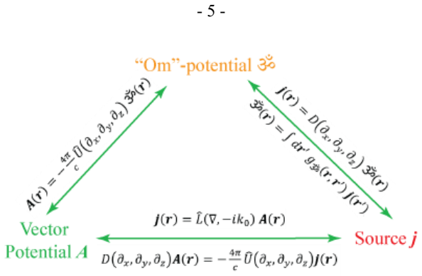
The central object is the Helmholtz operator for isotropy-broken media, $\hat{L}(i\boldsymbol{k},-ik_0)$, whose determinant $|\hat{L}|$ and adjoint $\operatorname{adj}\hat{L}$ are expanded through the Tamm-Rubilar tensor into two constant-coefficient differential operators $\hat{D}$ and $\hat{U}$ (the paper's Eqs. (9a)-(9b)). Since $\hat{D}$ and $\hat{U}$ commute in homogeneous media, the relation $\hat{D}\boldsymbol{A} = -\frac{4\pi}{c}\,\hat{U}\boldsymbol{j}$ factors through the intermediate 'Om' field $\boldsymbol{\text{ॐ}}$, with $\boldsymbol{j} = \hat{D}\,\boldsymbol{\text{ॐ}}$ and $\boldsymbol{A} = -\frac{4\pi}{c}\,\hat{U}\,\boldsymbol{\text{ॐ}}$. The leverage is that fixing ॐ (or fixing $\boldsymbol{A}$) puts all material dependence into $\hat{D}$ and $\hat{U}$, producing cross-material mappings of source-potential pairs; the paper uses Hermite functions as test fields and introduces a scalar 'Om' Green's function $g_{\text{ॐ}}$ for recovering ॐ from an arbitrary source.
What would settle it
A concrete numerical test: for a fixed homogeneous bianisotropic medium, generate many smooth distributed sources, compute the vector potential from Eq. (5), and check whether the pair satisfies Eqs. (11)-(12) for some Om field; any square-integrable source for which no such Om field exists — for instance because the scalar Om Green's function integral $g_{\text{ॐ}} = \int \frac{d^3k}{(2\pi)^3}\,|\hat{L}|^{-1}\,e^{i\boldsymbol{k}\cdot\boldsymbol{r}}$ fails to converge when the source spectrum does not vanish on the isofrequency surface $|\hat{L}| = 0$ — would falsify the claim that Eqs. (11)-(12) produce all valid current-potential pairs.
Extended reading notes
Core claim
On the paper's own terms, the dyadic Green's function is not the natural building block for macroscopic electromagnetism, and solutions for distributed sources can be built directly. In the inverse Helmholtz method, any chosen vector potential $\boldsymbol{A}(\boldsymbol{r})$ is assigned a source by direct application of the wave operator, $\boldsymbol{j}(\boldsymbol{r}) = \hat{L}(\nabla,-ik_0)\boldsymbol{A}(\boldsymbol{r})$. In the Om potential method, an auxiliary vector field $\boldsymbol{\text{ॐ}}(\boldsymbol{r})$ generates both the source, $\boldsymbol{j}(\boldsymbol{r}) = \hat{D}\,\boldsymbol{\text{ॐ}}(\boldsymbol{r})$, and the vector potential, $\boldsymbol{A}(\boldsymbol{r}) = -\frac{4\pi}{c}\,\hat{U}\,\boldsymbol{\text{ॐ}}(\boldsymbol{r})$, where $\hat{D}$ and $\hat{U}$ are constant-coefficient differential operators built from the determinant and adjoint of the Helmholtz operator $\hat{L}$; because they commute in homogeneous media, every chosen Om field yields a valid current and vector-potential pair. The paper demonstrates both constructions on Hermite-function test fields in a material family that passes through non-, mono-, bi-, tri-, and tetra-hyperbolic phases, showing how the required sources deform and rotate across the transitions.
Load-bearing premise
The construction hinges on the two differential operators having constant coefficients so that they commute, which holds only in homogeneous media, and it assumes without proof that every source distribution can be written as a fixed differential operator acting on some Om field.
Editorial extensions
If this is right
- In any homogeneous isotropy-broken medium, a chosen smooth vector potential determines a valid source by direct operator application, $\boldsymbol{j} = \hat{L}\boldsymbol{A}$, turning source-finding into a direct operator step rather than an integral over point sources.
- Any chosen Om field yields a valid source and vector potential, parameterizing a new space of solutions of macroscopic Maxwell's equations.
- The same vector potential can be produced in different media by correspondingly transformed sources, and the same Om field maps source-potential pairs as the material crosses topological transitions between hyperbolic phases.
- In vacuum the Om potential of a point source is a spherical wave propagating from the source, so the construction reproduces standard radiation behavior as a special case.
- For a fixed Om field, the pair $(\boldsymbol{j},\boldsymbol{A})$ can be tracked across material symmetry and topology changes using only the operators $\hat{D}$ and $\hat{U}$, without recomputing dyadic Green's functions.
Reading between the lines
- The exactness of the Om construction rests on $\hat{D}$ and $\hat{U}$ commuting; extending the same factorization to inhomogeneous or nonlocal media would require an operator-ordering prescription or a generalized Om Green's function, a natural next step the paper leaves open.
- Because the method fixes the field first and reads off the source, it is naturally an inverse-design tool: it could prescribe source distributions that generate a target near field in hyperbolic media, a use the paper leaves implicit.
- The paper's philosophical objection to point sources in macroscopic electromagnetism is separable from its mathematics; the testable content is that the singular burden moves from the dyadic Green's function to the scalar factor $1/|\hat{L}|$, and whether the scalar Om Green's function is genuinely easier to evaluate remains an open question.
- A quantitative comparison against the truncated eigenfunction-series method the paper cites as cumbersome would settle whether the Om route offers a practical speedup for the same bianisotropic problem; the paper demonstrates existence of solutions, not computational advantage.
Editorial analysis
A structured set of objections, weighed in public.
Referee Report
Summary. The manuscript claims to introduce two Green's-function-free methods for macroscopic electromagnetism in isotropy-broken media: the inverse Helmholtz equation method and the 'Om'-potential method. It defines a scalar differential operator D from the determinant |L̂| and an operator U from the adjugate of the Helmholtz operator L̂, proposes j = D Om and A = -(4π/c) U Om for an arbitrary vector field Om, and also proposes j = L̂ A for an arbitrary vector potential A. The paper illustrates these constructions with Hermite-function examples and maps the resulting sources and potentials as a material parameter κ is varied through topological transitions.
Significance. The algebraic identity underlying Eq. (10) is a correct transcription of the cofactor relation L̂ adj L̂ = |L̂| I for homogeneous media, and the Hermite-function examples are explicit and reproducible. However, the paper's central claim that solutions can be obtained without Green's functions is not supported: the Om method requires inversion of the scalar operator D via a scalar Green's function with the same spectral singularities as the original dyadic Green's function, and both proposed methods construct source/field pairs rather than solving for prescribed sources. The vacuum specialization also contains a sign error in the adjugate. These are load-bearing defects, not presentation issues.
major comments (4)
- [§3, Eqs. (10)-(12)] The central claim that the Om method bypasses Green's functions is contradicted by the manuscript's own inversion formula. For a prescribed source j, Eq. (11) must be inverted; the text gives Om(r) = ∫ dr' g_Om(r,r') j(r'), with g_Om(r,r') = ∫ d³k/(2π)³ (1/|L̂|) exp(ik·(r-r')). This is a scalar Green's function whose poles lie on exactly the same dispersion surfaces as the original dyadic Green's function because |L̂| is the determinant. Thus the method replaces one Green's function by another and does not avoid Green's-function convolutions for arbitrary sources.
- [§3, vacuum display] The vacuum adjugate is incorrect. For L̂(ik,-ik0) = kk + (k0²-k²)I, the adjugate is (k²-k0²)(kk - k0²I), equivalently (k0²-k²)(k0²I - kk), not (k²-k0²)(kk + k0²I). Consequently the stated U_vac = (∇²+k0²)(k0²I - ∇∇) has the wrong sign on the gradient-gradient term; the correct operator is (∇²+k0²)(∇∇ + k0²I). This error propagates into the vacuum specialization of Eq. (10) and the point-source example that follows.
- [§3-§4, Eqs. (11)-(13)] The proposed methods are parameterizations rather than solution methods. Eq. (13) defines the source as L̂ A for an arbitrarily chosen A, which is tautologically satisfied; Eqs. (11)-(12) generate a source and potential from an arbitrary Om, guaranteeing Eq. (10) by construction. Consequently the cross-material mappings in Figs. 3-4 are consequences of the chosen Ansatz, not independent predictions, and the conclusion that 'solutions to problems of macroscopic electromagnetism can be found' is unsupported for problems with prescribed sources.
- [§3, Eq. (9)] The method is restricted to homogeneous media. The operators D and U are defined with constant coefficients, and the paper notes they commute 'in homogeneous media'; no construction is given for inhomogeneous or nonlocal media. This contradicts the abstract's and introduction's promise of 'generic isotropy-broken media' and arbitrary environments, and it is not a trivial extension because the factorization |L̂|^{-1} adj L̂ underlying Eq. (10) is a Fourier-space, translation-invariant statement.
minor comments (4)
- [§3, Eq. (6) numbering] Equation numbering should be renumbered: the vacuum operator properties are labelled (6), duplicating the earlier Eq. (6).
- [Section 5 heading] The final section heading appears as '1. The Om-potential Method' although it should be '5.'; the section numbering is inconsistent.
- [Throughout, Eq. (5)] The text says 'adjoint operator' where 'adjugate' is meant; the cofactor matrix adj L̂ satisfies L̂ adj L̂ = |L̂| I, not the Hermitian adjoint.
- [§3, point-source example] The point-source example at the end of §3 uses the identity (∇²+k0²)[e^{ik0R}/(4πR)] = e^{ik0R}/(4πR), but the correct action on the Helmholtz spherical wave is -δ(r); this displayed equality should be corrected or removed.
Circularity Check
The Om and inverse-Helmholtz methods are parameterizations: they generate source/field pairs from a chosen Om or A by definition, and for prescribed sources the 'Om Green's function' reintroduces the exact inversion the paper claims to bypass.
-
self definitional
[Sec. 3, Eqs. (10)-(12)]
"Instead of representing the source 𝒋(𝒓) as a superposition of point charges as is done in the Green’s function method, we express the source via the underlying “Om” ॐ potential vector field 𝒋(𝒓) = 𝐷(𝜕𝑥, 𝜕𝑦, 𝜕𝑧) ॐ(𝒓), (11) From Eq. (10) an expression for the vector potential corresponding to source current Eq. (11) can be obtained as 𝑨(𝒓) = −4𝜋/𝑐 𝑈̂(𝜕𝑥, 𝜕𝑦, 𝜕𝑧) ॐ(𝒓) (12)"
Eqs. (11) and (12) are not derived from an independent source; they are constitutive definitions of j and A in terms of the arbitrarily chosen vector field Om. Substituting (11) into (10) forces (12) whenever D and U commute, so the constructed pair (j,A) satisfies the wave equation by construction. The cross-material mappings shown in Fig. 4 are therefore just the same Om acted on by different material operators, direct consequences of the definitions rather than independently predicted relations. The conclusion that this provides 'a broad new space of solutions' is a parameterization, not a derivation of fields from specified sources, and any displayed 'result' is true by construction.
-
other
[Sec. 3, after Eq. (12)]
"Note that for arbitrary source the underlying “Om” vector field ॐ(𝒓) can be found as ॐ(𝒓) = ∫ 𝑑𝒓′ 𝑔ॐ(𝒓, 𝒓′) 𝒋(𝒓′), where the scalar “Om” Green’s function is 𝑔ॐ(𝒓, 𝒓′) = ∫ 𝑑3𝑘/(2𝜋)3 1/|𝐿̂| exp(𝑖𝒌(𝒓 − 𝒓′))"
To handle a prescribed source, the paper defines the Om field by convolving j with a scalar Green's function whose Fourier kernel is 1/|L|. This is exactly the inverse of the same operator L whose dyadic Green's function, Eq. (7), has denominator |L|, so the alleged bypass of Green's functions reduces to replacing the dyadic Green's function with a scalar one. The subsequent field A = -(4π/c)U Om is obtained only after performing the same spectral inversion that GFM requires. Thus the headline claim that solutions can be found 'without the use of Green's functions' is contradicted by the paper's own formula for g_Om; for arbitrary sources the Om method is, by construction, a Green's-function method.
1 more flagged steps
-
renaming known result
[Sec. 4, Eq. (13)]
"The first method to find solutions of Eq. (5) relies on inverse approach to the Helmholtz equation 𝒋(𝒓) = 𝐿̂(∇, −𝑖𝑘0) 𝑨(𝒓), (13), where instead of looking for vector potential 𝑨(𝒓) for a given source 𝒋(𝒓), we set the vector potential 𝑨(𝒓) and obtain sources 𝒋(𝒓), which create the desired vector potential."
Eq. (13) is just the original wave equation (3a) rearranged to give the source in terms of the potential. It assigns a source to any chosen A rather than solving for A from a specified j, so it cannot support the stated goal of predicting fields of arbitrary charge distributions. The 'inverse method' is a definitional identity, not an independent derivation, and its outputs, e.g. Eq. (14), are direct operator evaluations on a chosen trial field.
full rationale
The paper's two 'methods' are constructions: for every Om, Eqs. (11)-(12) manufacture a current and a vector potential that satisfy Eq. (10); for every A, Eq. (13) manufactures a source. These are valid identities, but they do not predict anything beyond the definitions: the displayed cross-material mappings are obtained by applying material-dependent operators to the same chosen trial field. The central conclusion that GFM is bypassed is additionally undercut by the paper's own statement that an arbitrary source requires Om(r)=∫dr' g_Om(r,r')j(r'), i.e. a scalar Green's function with the same 1/|L| spectral kernel as the dyadic Green's function of Eq. (7). No external benchmarks or independent experimental checks are involved, so the illustrative plots cannot provide independent support. The homogeneity restriction (constant-coefficient D and U) is a real limitation but is secondary; even in homogeneous media the bypass claim fails for prescribed sources. No load-bearing self-citation chain is present; Refs. [13,14] supply the topological classification used only to label the parameter scans. The score is high because the central 'results' reduce by construction to the definitions of j and A in terms of Om or A, rather than being derived from independent inputs.
Assumptions & free parameters
free parameters (2)
- Hermite function widths w_x, w_y, w_z =
not given; treated as a common width w in figures
- Material matrix M entries =
not provided in text; color-coded in Fig. 2(e)
assumptions (6)
- standard math Maxwell's equations with constitutive relations (Eqs. 1-2) are the governing equations.
- standard math For an invertible matrix L, L^{-1} = adj(L)/det(L), Cramer's rule.
- domain assumption The media are homogeneous, so D and U have constant coefficients and commute.
- domain assumption Fields are time-harmonic and use the Weyl gauge, so B = ∇×A and E = -(1/c)∂_t A.
- domain assumption The scalar operator D is invertible on the source space, giving Om = ∫ g_Om j.
- ad hoc to paper Point sources and singular fields are not logically sound in macroscopic electromagnetism.
invented entities (1)
-
Om-potential ॐ(r)
Cite this review
Pith. "Pith review of Om-Theory of Macroscopic Electromagnetism: Greener Vibes for Isotropy-Broken Media." pith.science (2026). https://pith.science/paper/JSPMOVTB
@misc{pith2026250604393,
  author       = {Pith},
  title        = {Pith review of: Om-Theory of Macroscopic Electromagnetism: Greener Vibes for Isotropy-Broken Media},
  year         = {2026},
  howpublished = {\url{https://pith.science/paper/JSPMOVTB}},
  note         = {Machine review of arXiv:2506.04393}
}
read the original abstract
The applicability ranges of macroscopic and microscopic electromagnetisms are opposite. While microscopic electromagnetism deals with point sources, singular fields, and discrete atomistic materials, macroscopic electromagnetism concerns smooth average distributions of sources, fields, and homogenized effective metamaterials. Greens function method - GFM - involves finding fields of point sources and applying superposition principle to find fields of distributed sources. When utilized to solve microscopic problems GFM is perfectly within the applicability range. Extension of GFM to simple macroscopic problems is convenient, but not fully logically sound, since point sources and singular fields are technically not a subject of macroscopic electromagnetism. This explains the difficulty of both finding the Greens functions and applying superposition principle in complex isotropy-broken media, which are very different from microscopic environments. In this manuscript, we lay out a path to solution of macroscopic Maxwells equations for distributed sources bypassing GFM, by introducing inverse approach and a method based on Om-potential which we describe here. To the researchers of electromagnetism this provides access to powerful analytical tools and a broad new space of solutions for Maxwells equations.
Figures


Figures from the paper (1 more)

Reference graph
Works this paper leans on
-
[1]
Introduction to electrodynamics ,
D. J. Griffiths, “Introduction to electrodynamics ,” (Cambridge University Press, 202 3)
-
[2]
The classical theory of fields,
L. D. Landau, E. M. Lifshitz, “The classical theory of fields,” V ol. 2. (Nauka, Moscow, 1988)
work page 1988
-
[3]
The greening of quantum field theory: George and I,
J. Schwinger, “The greening of quantum field theory: George and I,” In Julian Schwinger: The Physicist, the Teacher, and the Man, pp. 13-27 (1996)
work page 1996
-
[4]
Nonlocal homogenization theory of structured materials ,
M. G. Silveirinha, “Nonlocal homogenization theory of structured materials ,” In Theory and Phenomena of Metamaterials ed. F. Capolino (CRC press, Boca Raton, FL, 2009)
work page 2009
-
[5]
Theorems of bianisotropic media ,
J. A. Kong, “Theorems of bianisotropic media ,” Proceedings of the IEEE 60(9) 1036 (1972)
work page 1972
-
[6]
Theory of electromagnetic waves: a coordinate -free approach,
H. C. Chen, “Theory of electromagnetic waves: a coordinate -free approach,” (McGraw Hill, 1983)
work page 1983
-
[7]
Infinite-space dyadic green functions in electromagnetism ,
M. Faryad, A . Lakhtakia, “ Infinite-space dyadic green functions in electromagnetism ,” (Morgan & Claypool Publishers, 2018 )
work page 2018
-
[8]
Electromagnetic Scattering by Bianisotropic Spheres ,
M. Durach, “Electromagnetic Scattering by Bianisotropic Spheres ,” Applied Sciences 13(8) 5169 (2023)
work page 2023
Show all 14 references
-
[9]
Principles of optics: electromagnetic theory of propagation, interference and diffraction of light ,
M. Born, E. Wolf, “Principles of optics: electromagnetic theory of propagation, interference and diffraction of light ,” (Elsevier, 2013)
2013
-
[10]
Beltrami fields in chiral media
A. Lakhtakia, “Beltrami fields in chiral media ” (World Scientific, 1994)
1994
-
[11]
Linear pre-metric electrodynamics and deduction of the light cone,
G. F. Rubilar, “Linear pre-metric electrodynamics and deduction of the light cone,” Ann. Phys. 514, 717 (2002) - 10 -
2002
-
[12]
Foundations of Classical Electrodynamics -Charge, Flux, and Metric,
F. W. Hehl, Y. N. Obukhov, “Foundations of Classical Electrodynamics -Charge, Flux, and Metric,” (Birkhauser: Boston, MA, USA, 2003)
2003
-
[13]
Tri-and tetrahyperbolic isofrequency topologies complete classification of bianisotropic materials ,
M. Durach, R. F. Williamson, M. Laballe, T. Mulkey, “Tri-and tetrahyperbolic isofrequency topologies complete classification of bianisotropic materials ,” Appl. Sci. 10, 763 (2020)
2020
-
[14]
M. Durach, “Tetra-hyperbolic and tri-hyperbolic optical phases in anisotropic metamaterials without magnetoelectric coupling due to hybridization of plasmonic and magnetic Bloch high -k polaritons,” Opt. Commun 476, 126349 (2020)
2020
Reviewed August 7, 2026 · model on record in the stance chip above.
Discussion (0). Continue with ORCID to comment.