REVIEW 1 major objections 5 minor 32 references
Strong stability of linear delay-difference equations
T0 review · 1 major / 5 minor · reviewed 2026-08-07 · deepseek-v4-flash
Pith's one-line read For scalar linear delay-difference equations, strong stability is equivalent to the total variation of the defining measure being less than 1.
desk verdict A clean, genuine extension of Melvin's criterion to distributed delays; the load-bearing citation worry is a non-issue. read the letter →
The pith
A machine-rendered reading of the paper's core claim, the machinery that carries it, and where it could break.
The reading
What carries the argument
The central object is the scalar total variation $\int_{-1}^0 d|\mu|$ of the matrix-valued Borel measure $\mu$ defining the delay term, since this single number separates strong stability from its failure for scalar equations. The argument's machinery includes the Hahn–Jordan decomposition, which splits $\mu$ into positive and negative parts to construct piecewise-constant rearrangement maps $\varphi$ with rationally independent delays; the Hale–Silkowski Criterion, which decides exponential stability of the resulting finite point-delay systems; and a cited trajectory-based lemma converting the pointwise bound $|x(t)|\le L\|x_t\|_\infty$ with $L<1$ into exponential stability.
What would settle it
A concrete disproof would be a bounded-variation scalar measure with $\int_{-1}^0 d|\mu| < 1$ and an admissible Borel map $\varphi$ for which the characteristic equation of the perturbed system (6) has a root in the closed right half-plane.
Extended reading notes
Core claim
Theorem 11 states that, for $n=1$, the following are equivalent: the total variation of the measure associated with $M$ satisfies $\int_{-1}^0 d|\mu|(\xi) < 1$; system (1) is locally strongly stable; and system (1) is strongly stable. Strong stability means exponential stability for every Borel-measurable map $\varphi:[-1,0]\to[-1,0]$ such that the pushed-forward measure $\varphi_*\mu$ is admissible, and local strong stability means the same for all $\varphi$ close to the identity in the uniform norm. The proof of the nontrivial implications uses the Hale–Silkowski Criterion for pointwise-delay systems to show that total variation at least 1 produces an unstable nearby system, and a trajectory-wise bound together with a cited lemma to show that total variation below 1 forces exponential stability of every admissible perturbation.
Load-bearing premise
The proof of the direction 'total variation less than 1 implies strong stability' assumes that the cited trajectory-based stability lemma applies to the continuous solutions of the pushed-forward equation, and that every admissible perturbation keeps the system well-posed through $\varphi_*\mu\in W$; if either fails, that implication is unsupported.
Editorial extensions
If this is right
- For any scalar equation of the form (1), checking strong stability reduces to one scalar: the total variation of the delay measure on $[-1,0]$ must be less than 1.
- Local and global strong stability are equivalent in the scalar case, so stability under all sufficiently small delay perturbations implies stability under every admissible Borel-measurable rearrangement of the delays.
- When the delay measure is a finite sum of point masses, the criterion becomes $\sum_k |A_k| < 1$, recovering Melvin's Criterion for pointwise-delay equations.
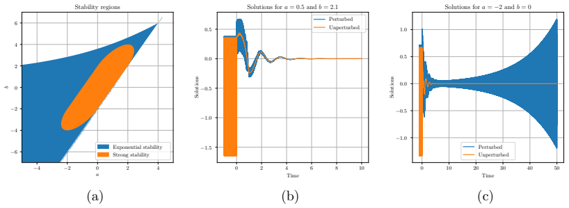
- The affine-density example yields an explicit strong-stability region in the $(a,b)$-plane, and the numerical comparison shows that exponential stability alone does not imply strong stability.
- Proposition 6 establishes global existence and uniqueness for the $n$-dimensional equation under the condition $\det(I-A_M)\ne 0$, so the stability analysis rests on a well-posed solution theory.
Reading between the lines
- The paper leaves the multi-dimensional case open; by analogy with (4), a natural candidate would be a spectral-radius condition such as $\sup_{\theta}\rho\!\left(\int_{-1}^0 e^{i\theta}\,dM(\theta)\right) < 1$.
- Because the definition quantifies over all Borel-measurable maps, total variation rather than finer spectral data is the decisive quantity for this very demanding stability notion.
- A testable byproduct is that random piecewise-constant delay rearrangements with rationally independent values should destabilise any scalar system whose total variation is at least 1, matching the construction in the proof.
Editorial analysis
A structured set of objections, weighed in public.
Referee Report
Summary. This paper considers linear delay-difference equations of the form (1), x(t)=∫_{-1}^0 dM(θ)x(t+θ), with M a matrix-valued function of bounded variation. It establishes a well-posedness result for this class (Proposition 6), recalls the Hale–Silkowski criterion for pointwise-delay systems (Theorem 8), and proposes a definition of strong stability for the distributed-delay setting by allowing Borel-measurable perturbations of the delay, i.e., replacing θ by φ(θ) in the integral (Definition 9). The main result (Theorem 11) states that, in the scalar case n=1, local strong stability, global strong stability, and the total variation condition ∫d|µ|<1 are equivalent. The paper also provides numerical examples illustrating the region of strong stability for an affine density and comparing it with the region of exponential stability.
Significance. Should the main theorem hold, the paper gives a strikingly simple and parameter-free characterization of robust stability for scalar distributed-delay difference equations: the only quantity that matters is the total variation of the measure. The necessity direction is elegant, combining Hahn–Jordan decomposition with a partition argument that reduces the problem to the classical Hale–Silkowski criterion; the sufficiency direction uses a pointwise inequality and a cited lemma. The paper also contains a useful well-posedness theorem and numerical experiments that clearly exhibit the gap between exponential stability and strong stability. The result has the potential to be useful in applications to hyperbolic PDEs with in-domain couplings, where distributed delay terms arise naturally.
major comments (1)
- [Section 3.3, proof of Theorem 11 (direction 1⇒3)] The proof of the direction 1⇒3 in Theorem 11 is the only load-bearing step that is not proved in detail: it consists of the sentence 'Hence, from [24, Lemma 1], (6) is exponentially stable.' The manuscript neither states the lemma nor verifies that the continuous solutions of (6) satisfy its hypotheses. In particular, if φ*µ has an atom at 0, then (6) contains an instantaneous term and the inequality |x(t)|≤L‖x_t‖∞ (with L<1) does not by itself put the system in the standard small-gain form without extra reasoning. Since this is the sole argument for global strong stability under condition (7), the proof is incomplete as written. The gap is readily fixable by either quoting the lemma explicitly with all hypotheses or by giving a direct induction on unit intervals, which would also handle the atom-at-zero case; the claim itself is very likely correct.
minor comments (5)
- [Section 3.3, proof of Theorem 11] The notation −τP k and −τN k is typeset in a way that makes the indices unclear; please use a clearer notation such as −τ_{P,k} and −τ_{N,k}.
- [Section 3, Definition 3] The partition of [a,b] is written as {[t_i,t_{i+1}] : 1≤i≤k}; it would be clearer to state explicitly that t_0=a and t_{k+1}=b.
- [Section 4.1] The computation of Var M|_{[-1,0]} for the affine density would be easier to follow if the cases b=0 and b≠0 were treated separately, with the convention θ_v=0 for b=0 stated as a limiting case.
- [Section 4.2] The norm ∥·∥_2 used in the definition of α is not defined; please specify that it is the induced Euclidean norm, or state that the bounds are norm-independent.
- [Section 2, proof of Proposition 6] After the change of variables from M to N, it would be helpful to explicitly note that N has no atom at 0, so that det(I−A_N)=1 and the contraction argument applies.
Circularity Check
No significant circularity: the main criterion is a parameter-free condition on the measure, and the proof invokes external theorems rather than assuming its conclusion.
full rationale
The derivation in Theorem 11 is self-contained with respect to the paper's own claims. Statement (1) is a scalar quantity, the total variation of the measure mu, which is not fitted to the stability property being proved. The direction (2) implies (1) explicitly constructs, via Hahn-Jordan decomposition, a perturbed system with pointwise delays whose Hale-Silkowski spectral radius is at least 1 whenever the total variation is at least 1, so instability is derived from an external criterion, not assumed. The direction (1) implies (3) relies on the pointwise inequality |x(t)| <= L ||x_t||_infty with L = integral d|mu| < 1, and then cites the external Mazenc-Malisoff lemma [24, Lemma 1] to conclude exponential stability. That lemma is an independent published result, not derived from the present paper, and no parameter of the paper is fitted to make the inequality hold. The authors' own works appear only in contextual citations and are not load-bearing in the proof. The only notable concern is that the hypotheses of [24, Lemma 1] are not stated or verified in the paper, but that is a completeness or correctness risk, not circularity, because the cited lemma does not presuppose the theorem being proved.
Assumptions & free parameters
assumptions (6)
- standard math M is a normalized right-continuous matrix-valued function of bounded variation, with the measure correspondence of Remark 5.
- domain assumption M belongs to W, that is det(I - A_M) is nonzero with A_M = M(0) - M(0-).
- standard math Hale-Silkowski Criterion (Theorem 8), attributed to Avellar-Hale [2] and Silkowski [29].
- standard math Mazenc-Malisoff Lemma [24, Lemma 1].
- standard math Hahn and Jordan decomposition of signed measures.
- standard math Characteristic equation criterion for exponential stability of delay equations, from Hale [16].
Cite this review
Pith. "Pith review of Strong stability of linear delay-difference equations." pith.science (2026). https://pith.science/paper/FPOW56QL
@misc{pith2026250605002,
  author       = {Pith},
  title        = {Pith review of: Strong stability of linear delay-difference equations},
  year         = {2026},
  howpublished = {\url{https://pith.science/paper/FPOW56QL}},
  note         = {Machine review of arXiv:2506.05002}
}
read the original abstract
This paper considers linear delay-difference equations, that is, equations relating the state at a given time with its past values over a given bounded interval. After providing a well-posedness result and recalling Hale--Silkowski Criterion for strong stability in the case of equations with finitely many pointwise delays, we propose a generalization of the notion of strong stability to the more general class of linear delay-difference equations with an integral term defined by a matrix-valued measure. Our main result is an extension of Melvin Criterion for the strong stability of scalar equations, showing that local and global strong stability are equivalent, and that they can be characterized in terms of the total variation of the function defining the equation. We also provide numerical illustrations of our main result.
Figures
Reference graph
Works this paper leans on
-
[1]
J. Auriol and F. Di Meglio. An explicit mapping from linear first order hyperbolic PDEs to difference systems. Systems Control Lett. , 123:144–150, 2019
work page 2019
-
[2]
C. E. Avellar and J. K. Hale. On the zeros of exponential polynomials. J. Math. Anal. Appl. , 73(2):434–452, 1980
work page 1980
-
[3]
I. Balogoun, J. Auriol, I. Boussaada, and G. Mazanti. A novel necessary and sufficient con- dition for the stability of 2 × 2 first-order linear hyperbolic systems. Systems Control Lett. , 199:Paper No. 106066, 9, 2025
work page 2025
-
[4]
R. Bellman and K. L. Cooke. Differential-difference equations. Academic Press, 1963
work page 1963
-
[5]
R. K. Brayton. Bifurcation of periodic solutions in a nonlinear difference-differential equations of neutral type. Quart. Appl. Math. , 24:215–224, 1966
work page 1966
-
[6]
Y. Chitour, S. Marx, and G. Mazanti. One-dimensional wave equation with set-valued bound- ary damping: well-posedness, asymptotic stability, and decay rates. ESAIM Control Optim. Calc. Var., 27:Paper No. 84, 62, 2021. 9
work page 2021
-
[7]
Y. Chitour, G. Mazanti, and M. Sigalotti. Stability of non-autonomous difference equations with applications to transport and wave propagation on networks. Netw. Heterog. Media , 11(4):563–601, 2016
work page 2016
-
[8]
Y. Chitour, G. Mazanti, and M. Sigalotti. Persistently damped transport on a network of circles. Trans. Amer. Math. Soc. , 369(6):3841–3881, 2017
work page 2017
Show all 32 references
-
[9]
K. L. Cooke and D. W. Krumme. Differential-difference equations and nonlinear initial- boundary value problems for linear hyperbolic partial differential equations. J. Math. Anal. Appl., 24:372–387, 1968
1968
-
[10]
Coron, G
J.-M. Coron, G. Bastin, and B. d’Andr´ ea Novel. Dissipative boundary conditions for one- dimensional nonlinear hyperbolic systems. SIAM J. Control Optim. , 47(3):1460–1498, 2008
2008
-
[11]
M. Cruz, A. and J. K. Hale. Stability of functional differential equations of neutral type. J. Differential Equations, 7:334–355, 1970
1970
-
[12]
Diekmann, S
O. Diekmann, S. A. van Gils, S. M. Verduyn Lunel, and H.-O. Walther. Delay equations: Functional, complex, and nonlinear analysis , volume 110 of Applied Mathematical Sciences . Springer-Verlag, 1995
1995
-
[13]
G. B. Folland. Real analysis: Modern techniques and their applications . Pure and Applied Mathematics (New York). John Wiley & Sons, second edition, 1999
1999
-
[14]
Fridman, S
E. Fridman, S. Mondi´ e, and B. Saldivar. Bounds on the response of a drilling pipe model. IMA J. Math. Control Inform. , 27(4):513–526, 2010
2010
-
[15]
Gugat and M
M. Gugat and M. Sigalotti. Stars of vibrating strings: switching boundary feedback stabiliza- tion. Netw. Heterog. Media, 5(2):299–314, 2010
2010
-
[16]
J. Hale. Theory of functional differential equations, volume 3 ofApplied Mathematical Sciences. Springer-Verlag, second edition, 1977
1977
-
[17]
J. K. Hale. Parametric stability in difference equations. Boll. Un. Mat. Ital. (4) , 11(3):209–214, 1975
1975
-
[18]
J. K. Hale, E. F. Infante, and F. S. P. Tsen. Stability in linear delay equations. J. Math. Anal. Appl., 105(2):533–555, 1985
1985
-
[19]
J. K. Hale and S. M. Verduyn Lunel. Introduction to functional-differential equations , vol- ume 99 of Applied Mathematical Sciences. Springer-Verlag, 1993
1993
-
[20]
J. K. Hale and S. M. Verduyn Lunel. Strong stabilization of neutral functional differential equations. IMA J. Math. Control Inform. , 19(1-2):5–23, 2002. Special issue on analysis and design of delay and propagation systems
2002
-
[21]
D. Henry. Linear autonomous neutral functional differential equations. J. Differential Equa- tions, 15:106–128, 1974
1974
-
[22]
G.-D. Hu. Stability criteria of linear neutral systems with distributed delays. Kybernetika (Prague), 47(2):273–284, 2011
2011
-
[23]
G. Mazanti. Stability and stabilization of linear switched systems in finite and infinite dimen- sions. PhD thesis, ´Ecole Polytechnique, University Paris–Saclay, Palaiseau, France, September 2016
2016
-
[24]
Mazenc and M
F. Mazenc and M. Malisoff. Trajectory based approach for the stability analysis of nonlinear systems with time delays. IEEE Trans. Automat. Control , 60(6):1716–1721, 2015
2015
-
[25]
W. R. Melvin. Stability properties of functional difference equations. J. Math. Anal. Appl. , 48:749–763, 1974. 10
1974
-
[26]
Michiels and S.-I
W. Michiels and S.-I. Niculescu. Stability, control, and computation for time-delay systems: An eigenvalue-based approach, volume 27 of Advances in Design and Control . SIAM, second edition, 2014
2014
-
[27]
Michiels, T
W. Michiels, T. Vyhl ´ ıdal, P. Z ´ ıtek, H. Nijmeijer, and D. Henrion. Strong stability of neutral equations with an arbitrary delay dependency structure. SIAM J. Control Optim. , 48(2):763– 786, 2009
2009
-
[28]
C. J. Moreno. The zeros of exponential polynomials. Compositio Math., 26:69–78, 1973
1973
-
[29]
R. A. Silkowski. Star-shaped regions of stability in hereditary systems . PhD thesis, Division of Applied Mathematics, Brown University, 1976
1976
-
[30]
Sipahi, S.-I
R. Sipahi, S.-I. Niculescu, C. T. Abdallah, W. Michiels, and K. Gu. Stability and stabilization of systems with time delay: limitations and opportunities. IEEE Control Syst. Mag., 31(1):38– 65, 2011
2011
-
[31]
M. Slemrod. Nonexistence of oscillations in a nonlinear distributed network. J. Math. Anal. Appl., 36:22–40, 1971
1971
-
[32]
Vyhl ´ ıdal and P
T. Vyhl ´ ıdal and P. Z ´ ıtek. QPmR—quasi-polynomial root-finder: algorithm update and ex- amples. In Delay systems , volume 1 of Adv. Delays Dyn. , pages 299–312. Springer, Cham, 2014. 11
2014
Reviewed August 7, 2026 · model on record in the stance chip above.
Discussion (0). Sign in to comment.