REVIEW 3 major objections 8 minor 1 cited by
The Hourglass Simulation: A Catalog for the Roman High-Latitude Time-Domain Core Community Survey
T0 review · 3 major / 8 minor · reviewed 2026-08-07 · deepseek-v4-flash
Pith's one-line read Hourglass simulation predicts 64,000 transients for Roman survey
desk verdict Hourglass is a genuinely useful planning and training catalog for Roman time-domain work; the headline counts need rate-uncertainty bands, but that does not undercut its main value. read the letter →
The pith
A machine-rendered reading of the paper's core claim, the machinery that carries it, and where it could break.
The reading
What carries the argument
The machinery is a forward-modeling pipeline built on the SNANA simulation library, run through the PIPPIN pipeline manager, which turns rest-frame spectral-temporal energy distribution (SED) models into observed Roman light curves and prism spectra. Each of the ten transient classes is injected using a specific SED library — SALT3-NIR for SNe Ia, Vincenzi et al. (2019) models for core-collapse supernovae, MOSFiT-generated templates for superluminous supernovae, tidal disruption events, ILOTs, and pair-instability supernovae, the Bulla (2019) model for kilonovae, and the ELAsTiCc damped random walk model for AGN — with volumetric rates drawn from the literature and host galaxies from the 3DHST catalog. The pipeline then applies the survey geometry, filter transmissions, exposure times, PSF noise-equivalent areas, read noise, sky noise, and a 0.15 mag zero-point scatter, and retains objects with two epochs above S/N=5.
What would settle it
Measure the volumetric SN Ia rate in the 2<z<3 range — for instance with JWST slitless spectroscopy over a modest field — and compare it to the (1+z)^(-0.1) extrapolation used here; a rate significantly below that curve would falsify the predicted ~21,700 SNe Ia and the ~19,000 cosmologically useful subset proportionally.
Extended reading notes
Core claim
The central claim is that, under the current design-reference survey — a wide tier of 19.04 $deg^{2}$ in R/Z/Y/J, a deep tier of 4.20 $deg^{2}$ in Y/J/H/F, five-day cadence, two-year baseline, with roughly a fifth of the area covered by the R~100 prism — Roman will produce a science-independent time-domain catalog of over 64,000 transients detected at S/N>5 in two epochs. The simulation counts 21,700 Type Ia supernovae (about 19,000 with S/N at maximum above 10, the paper's proxy for cosmologically useful), 39,000 core-collapse supernovae, 1,300 SN1991bg-like events, 1,300 Type Iax supernovae, about 70 superluminous supernovae, 39 tidal disruption events, 35 intermediate-luminosity optical transients, 15 pair-instability supernovae, and 139 active galactic nuclei, with 14 kilonovae recovered from a simulation injected at five times the assumed true rate. The paper further claims these simulations are realistic enough to train machine-learning classifiers, and demonstrates this with a SCONE model that reaches 94% accuracy and 98% precision separating SNe Ia from contaminants; it also presents the first realistic prism spectral time series for non-Ia transients.
Load-bearing premise
The predicted catalog sizes scale linearly with input volumetric rates that are either extrapolated far beyond their measured redshift range (SN Ia and CCSN rates assumed valid to z=3) or uncertain by factors of 2–3 (kilonovae, pair-instability supernovae), so if those rates are wrong the headline counts change proportionally.
Editorial extensions
If this is right
- Roman's High-Latitude Time-Domain survey should deliver roughly an order of magnitude more Type Ia supernovae than current cosmological samples, with most of the ~19,000 cosmologically useful events lying above z=1.
- Core-collapse supernovae outnumber SNe Ia by almost two to one, making them the dominant source of contamination for photometric SN Ia classification and a key input for contamination studies.
- Rare transients will be detected in small but meaningful numbers — about 70 SLSNe, 39 TDEs, 15 PISNe, and ~3 kilonovae at the true rate — enough to begin constraining their rates and physics.
- The released simulated photometry, prism spectra, and input files give the community a testbed for survey optimization, classifier training, and selection-effect modeling before launch.
- Adopting the newer survey recommendations (larger deep tier, interweaving cadence, pilot and extended surveys) would raise the projected yield by about 25–30%, beyond 100,000 transients.
Reading between the lines
- Because every count scales linearly with the assumed volumetric rate, the Hourglass catalog can double as a forecast to be tested: the first year of real Roman data should resolve whether the z=2–3 extrapolation of the SN Ia and CCSN rates holds, and a single Roman kilonova would directly test the factor-of-five scaled injection rate.
- The 11,000 Å red edge of many SED models means the deep tier's H and F bands are effectively untested for low-redshift objects; extending the SED libraries redward would likely change predicted colors and classification performance in those bands.
- The same simulation structure could be extended to variable stars, Galactic sources, and rarer exotic transients to build a complete 'everything that varies' catalog for Roman, which would be the natural basis for alert-broker and anomaly-detection development.
- SCONE's precision drops noticeably beyond z≈2.5, suggesting that the highest-redshift SNe Ia — the most valuable for cosmology — are the hardest to classify photometrically; training on prism spectra or adding host-galaxy information is a natural next test.
Editorial analysis
A structured set of objections, weighed in public.
Referee Report
Summary. The paper presents the Hourglass simulation, an end-to-end forward simulation of the extragalactic time-domain catalog expected from the Roman High-Latitude Time-Domain Core Community Survey under the current reference design. The authors combine rest-frame SED templates and volumetric rate functions for ten transient classes (SNe Ia, SNIa-91bg, SNe Iax, CCSNe, SLSNe-I, TDEs, ILOTs, KNe, PISNe, and AGN) with the SNANA/PIPPIN simulation pipeline, a two-tier photometric survey (wide RZYJ, deep YJHF), prism spectroscopy, and a documented WFI noise model. The headline results are predicted catalog yields (approximately 21,700 SNe Ia, 39,000 CCSNe, 70 SLSNe-I, 39 TDEs, 14 KNe at five times the fiducial rate, 15 PISNe, and 139 AGN), a public data release of photometry, prism spectra, and object metadata, and a demonstration that the SCONE convolutional classifier reaches roughly 94% accuracy and 98% precision for photometrically classifying SNe Ia in these simulations.
Significance. If the adopted rates and SED models are accepted, this is a valuable community planning resource. Its strengths include a public data release with input files and catalog products, built on the well-tested SNANA and PIPPIN infrastructure, a forward-propagated simulation with no parameters fit to the output, and unusually transparent documentation of the survey geometry, instrument characteristics, and selection cuts. The paper also provides the first public simulated Roman prism spectral time series for several non-Ia classes, which is useful for pipeline development. The central weakness is that the headline yields are point predictions that inherit large, explicitly acknowledged input-rate uncertainties without any propagation, so the catalog cannot currently separate rate-driven variations from survey-design effects. The SCONE classifier results are a useful in silico benchmark, not a prediction of real-data performance, and the paper mostly frames them appropriately.
major comments (3)
- [§2.2, Table 1, §3.2] The headline yields in Table 4 are quoted as point values even though several input rates carry large, explicitly acknowledged uncertainties and are extrapolated beyond their measured ranges. Section 2.1.1 assumes the Strolger et al. (2020) SN Ia rate is valid to z=3 even though the majority of the 21,700 simulated SNe Ia lie at z>1 where that source reports significant uncertainty; Section 2.1.8 simulates KNe at five times the Abbott et al. (2021) rate, whose stated uncertainty is a factor of about three (up to four); Section 2.1.9 adopts a PISN rate that at z=1 is nearly twice the Pan et al. (2012) value. Section 4 acknowledges that "all of these results are highly dependent on the assumed rates," but Table 4 and the released catalog contain no uncertainty bands or sensitivity variants. Because the yields are linearly proportional to the adopted volumetric rates, users cannot separate rate-driven variation from survey-design effects. I request a sensitivity analysis (for example, rerunning with the upper and lower rate bounds for SNe Ia, KNe, and PISNe) and propagation of those bounds into Table 4 and the abstract's headline numbers.
- [§2.2, §3, Table 4] Several non-Ia SED models (CCSN, SLSN-I, TDE, ILOT, and PISN) have a rest-frame red edge of 11,000 Å (Table 1), while the Roman prism is transmissive to 18,000 Å and the deep tier includes H and F filters. The paper notes the J-band consequence in Section 2.2, but the abstract's claim of "the first realistic simulations of non-Type Ia supernovae spectral-time series data" is stronger than what these truncated SEDs can support, since at low redshift the reddest prism bins and the H/F photometry are not actually simulated for those classes. Please either extend the SEDs into the near-infrared (as was done for SNe Ia and SNIa-91bg), or explicitly quantify which fraction of objects and which wavelength bins are affected, and soften the "realistic" claim accordingly.
- [§2.2, §3, Table 4] The host-galaxy catalog limits the simulation to z<3, and the paper states that "significantly higher redshift PISN and SLSN will be visible" and that Hourglass only captures the low-redshift tail of these populations. Nevertheless, Table 4 lists PISN (15) and SLSN-I (70) as detected counts without flagging them as truncated lower limits in the table itself. Since Moriya et al. (2022) estimate on the order of 100 PISN at z>5, the z=3 cutoff is not a negligible edge effect for exactly the classes that appear in the abstract as "possibly pair-instability supernovae." Please mark these entries as lower limits and, if feasible, add an estimate of the unmodeled high-redshift contribution.
minor comments (8)
- [Abstract] There is a missing space in "theRoman High-Latitude Time-Domain Core Community Survey" in the abstract.
- [§2.1.10] The AGN volumetric rate is written as "1.0−3 Mpc−3"; this appears to be a formatting error for 1.0×10^-3 Mpc^-3 and should be corrected.
- [§2.1.9] The phrase "A volumetric rate for PISN presented stated in Briel et al. (2022)" contains a doubled verb; please revise.
- [Table 5] The column description for "mw_ebv" contains the typo "ling-of-sight" instead of "line-of-sight."
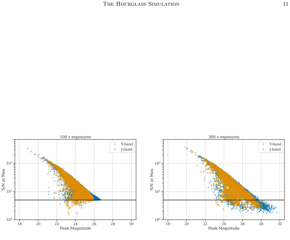
- [§2.2 and Abstract] The detection threshold is described as "two observations with S/N >5" in Section 2.2 but as "a S/N at max of >5" in the abstract; please clarify whether the requirement is two single-epoch detections at any phase, two detections near peak, or something else.
- [Figure 9] The horizontal axis of Figure 9 ends at z=2.5, while the text discusses a drop-off at z>2.5 and the simulation extends to z≈3; extending the axis would make the claimed high-redshift degradation visible.
- [§3.3] The SCONE precision and recall are measured on a test set generated with the same simulation machinery used for training. This is a legitimate in silico validation, but the caption and text should more prominently state that these numbers quantify simulation-to-simulation transfer, not expected performance on real Roman data.
- [Table 3] The header "ZPAVG" is a nonstandard abbreviation; consider defining it in the table caption or using the explicit expression from Equation (8).
Circularity Check
No circularity: Hourglass is a forward simulation; catalog yields are propagated from external rates, SED models, and a stated survey design, with the paper itself flagging the main rate uncertainties.
full rationale
The Hourglass catalog is produced by a forward chain: rest-frame SED templates and volumetric rates (Sections 2.1.1–2.1.10, Table 1) are redshifted, integrated through Roman filter and prism throughput curves, and passed through a noise model and a fixed S/N > 5 detection threshold (Sections 2.2–2.3). No parameter is fit to the catalog outputs, and the headline counts in Table 4 are not used as inputs anywhere in the simulation. The rate assumptions come from external measurements (Strolger et al. 2020, 2015; Prajs et al. 2017; Kochanek 2016; van Velzen 2018; Abbott et al. 2021; Briel et al. 2022), and the paper explicitly flags their uncertainty: SN Ia rates are extrapolated to z = 3 (Section 2.1.1), CCSN rates to z = 3 (Section 2.1.4), kilonovae are simulated at five times the Abbott et al. rate with a stated factor-of-~3 uncertainty (Section 2.1.8), and the PISN rate is roughly twice the Pan et al. value at z = 1 (Section 2.1.9). Section 4 states: 'All of these results are highly dependent on the assumed rates.' The survey design is taken from the authors' own reference-survey papers (Rose et al. 2021; Hounsell et al. 2023), but this is an explicitly stated modeling input rather than a result derived from the simulation, and the paper notes that the observational strategy is not finalized. The SCONE classification test (Section 3.3) trains and evaluates on the same simulated catalog; this is an in silico validation presented as such ('we train and test the binary classification of SCONE'), so it does not make the catalog derivation circular. The paper is self-contained as a forward simulation; the main caveats are rate-driven sensitivity and in-sample classifier validation, which are uncertainty and methodology concerns, not circularity.
Assumptions & free parameters
free parameters (3)
- Volumetric rate functions R(z) for each transient class =
SN Ia: 2.4e-5(1+z)^1.55 (z<1), 7.5e-5(1+z)^-0.1 (z>=1); KN: 3.2e-7 plus 5x simulation scale
- Fractional rates for subclasses (SNIa-91bg, SN Iax, ILOT) =
15% of SN Ia rate; 30% of SN Ia rate; 6% of CCSN rate
- Zero-point scatter =
0.15 mag rms
assumptions (4)
- domain assumption Flat Lambda-CDM cosmology with Omega_M=0.3, h=0.7
- ad hoc to paper Input SN Ia and CCSN volumetric rates measured at z<2 are valid when extrapolated to z=3
- domain assumption SED models are accurate over their stated wavelength ranges, including the red-edge cutoff at 11,000 Angstrom for several transient types
- domain assumption The Rose et al. (2021) reference survey design is representative of the eventual Roman survey
Cite this review
Pith. "Pith review of The Hourglass Simulation: A Catalog for the Roman High-Latitude Time-Domain Core Community Survey." pith.science (2026). https://pith.science/paper/VTV77MKZ
@misc{pith2026250605161,
  author       = {Pith},
  title        = {Pith review of: The Hourglass Simulation: A Catalog for the Roman High-Latitude Time-Domain Core Community Survey},
  year         = {2026},
  howpublished = {\url{https://pith.science/paper/VTV77MKZ}},
  note         = {Machine review of arXiv:2506.05161}
}
abstract
We present a simulation of the time-domain catalog for the Nancy Grace Roman Space Telescope's High-Latitude Time-Domain Core Community Survey. This simulation, called the Hourglass simulation, uses the most up-to-date spectral energy distribution models and rate measurements for ten extra-galactic time-domain sources. We simulate these models through the design reference Roman Space Telescope survey: four filters per tier, a five day cadence, over two years, a wide tier of 19 deg$^2$ and a deep tier of 4.2 deg$^2$, with $\sim$20% of those areas also covered with prism observations. We find that a science-independent Roman time-domain catalog, assuming a S/N at max of >5, would have approximately 21,000 Type Ia supernovae, 40,000 core-collapse supernovae, around 70 superluminous supernovae, $\sim$35 tidal disruption events, 3 kilonovae, and possibly pair-instability supernovae. In total, Hourglass has over 64,000 transient objects, 11 million photometric observations, and 500,000 spectra. Additionally, Hourglass is a useful data set to train machine learning classification algorithms. We show that SCONE is able to photometrically classify Type Ia supernovae with high precision ($\sim$95%) to a z > 2. Finally, we present the first realistic simulations of non-Type Ia supernovae spectral-time series data from Roman's prism.
Figures


Figures from the paper (5 more)


Forward citations
Cited by 1 Pith paper
-
A Simulation Based Inference Approach to Modelling of Type Ia Supernova Populations
A simulation-based inference pipeline (Stjörnumál) fits SN Ia dust and intrinsic scatter models to DES 5-year data, enabling fast Bayesian model comparison across seven SN Ia population models.
Reference graph
Works this paper leans on
- [1]
- [2]
- [3]
-
[4]
Briel, M. M., Eldridge, J. J., Stanway, E. R., Stevance, H. F., & Chrimes, A. A. 2022, 514, 1315
work page 2022
-
[5]
Casertano, S. 2022, Determining the Best-Fitting Slope and Its Uncertainity for up-the-Ramp Sampled Images with Unevenly Distributed Resultants, Nancy Grace Roman Space Telescope Technical Reports, 38 pp
work page 2022
- [6]
- [7]
-
[8]
2011, A&A, 529, L4, http://www.aanda.org/10.1051/0004-6361/201116723
Chotard, N., Gangler, E., Aldering, G., et al. 2011, A&A, 529, L4, http://www.aanda.org/10.1051/0004-6361/201116723
Show all 76 references
-
[9]
2012, 491, 228
Cooke, J., Sullivan, M., Gal-Yam, A., et al. 2012, 491, 228
2012
-
[10]
DeCoursey, C., Egami, E., Pierel, J. D. R., et al. 2025, 979, 250
2025
-
[11]
E., Villasenor, B., Robertson, B
Drakos, N. E., Villasenor, B., Robertson, B. E., et al. 2022, 926, 194
2022
-
[12]
V., Richmond, M
Filippenko, A. V., Richmond, M. W., Branch, D., et al. 1992, AJ, 104, 1543, https://ui.adsabs.harvard.edu/ #abs/1992AJ....104.1543F/abstract
1992
-
[13]
Fitzpatrick, E. L. 1999, 111, 63
1999
-
[14]
J., Challis, P
Foley, R. J., Challis, P. J., Chornock, R., et al. 2013, ApJ, 767, 57, http://stacks.iop.org/0004-637X/767/i=1/a=57? key=crossref.be847ca54941021d2dbe7cb5b7ddacc5
2013
-
[15]
Gal-Yam, A., & Leonard, D. C. 2009, 458, 865
2009
-
[16]
2023, Implementation of Unevenly Spaced Resultants in Pandeia, Nancy Grace Roman Space Telescope Technical Reports, 8 pp
Gomez, S. 2023, Implementation of Unevenly Spaced Resultants in Pandeia, Nancy Grace Roman Space Telescope Technical Reports, 8 pp
2023
-
[17]
2019, 881, 87 Gonz´ alez-Gait´ an, S., Perrett, K., Sullivan, M., et al
Gomez, S., Berger, E., Nicholl, M., et al. 2019, 881, 87 Gonz´ alez-Gait´ an, S., Perrett, K., Sullivan, M., et al. 2011, 727, 107 Gonz´ alez-Gait´ an, S., Hsiao, E. Y., Pignata, G., et al. 2014, 795, 142
2019
-
[18]
R., Rest, A., et al
Graur, O., Zurek, D. R., Rest, A., et al. 2017, arXiv:1711.01275, http://arxiv.org/abs/1711.01275
2017 arXiv
-
[19]
A., et al
Guillochon, J., Nicholl, M., Villar, V. A., et al. 2018, 236, 6
2018
-
[20]
2010, A&A, 523, A7, http://www.aanda.org/10.1051/0004-6361/201014468
Guy, J., Sullivan, M., Conley, A., et al. 2010, A&A, 523, A7, http://www.aanda.org/10.1051/0004-6361/201014468
2010 doi
-
[21]
R., Millman, K
Harris, C. R., Millman, K. J., van der Walt, S. J., et al. 2020, Nature, 585, 357, https://www.nature.com/articles/s41586-020-2649-2
2020
-
[22]
2020, JOSS, 5, 2122, https://joss.theoj.org/papers/10.21105/joss.02122
Hinton, S., & Brout, D. 2020, JOSS, 5, 2122, https://joss.theoj.org/papers/10.21105/joss.02122
2020 doi
-
[23]
J., et al
Hounsell, R., Scolnic, D., Foley, R. J., et al. 2018, ApJ, 867, 23, http://arxiv.org/abs/1702.01747
2018 arXiv
-
[24]
2023, arXiv e-prints, arXiv:2307.02670
Hounsell, R., Scolnic, D., Brout, D., et al. 2023, arXiv e-prints, arXiv:2307.02670
2023 arXiv
-
[25]
Hunter, J. D. 2007, CSE, 9, 90, http://ieeexplore.ieee.org/document/4160265/
2007
-
[26]
2024, ApJ, 966, 164, https: //iopscience.iop.org/article/10.3847/1538-4357/ad344c
Inayoshi, K., Kashiyama, K., Li, W., et al. 2024, ApJ, 966, 164, https: //iopscience.iop.org/article/10.3847/1538-4357/ad344c
2024 doi
-
[27]
Jha, S. W. 2017, arXiv:1707.01110, http://arxiv.org/abs/1707.01110
2017 arXiv
-
[28]
2001, Nature Methods, arXiv:1907.10121, http://www.scipy.org/
Jones, E., Oliphant, T., Peterson, P., et al. 2001, Nature Methods, arXiv:1907.10121, http://www.scipy.org/
2001 arXiv
-
[29]
2010, 717, 245
Kasen, D., & Bildsten, L. 2010, 717, 245
2010
-
[30]
2017, 551, 80
Ramirez-Ruiz, E. 2017, 551, 80
2017
-
[31]
E., & Heger, A
Kasen, D., Woosley, S. E., & Heger, A. 2011, 734, 102
2011
-
[32]
2017, ApJ, 836, 56, http://stacks.iop.org/0004-637X/836/i=1/a=56?key= crossref.d0bddb5607f63ec4347f7e1b0143aef5
Kessler, R., & Scolnic, D. 2017, ApJ, 836, 56, http://stacks.iop.org/0004-637X/836/i=1/a=56?key= crossref.d0bddb5607f63ec4347f7e1b0143aef5
2017
-
[33]
P., Cinabro, D., et al
Kessler, R., Bernstein, J. P., Cinabro, D., et al. 2009b, PASP, 121, 1028, http://iopscience.iop.org/article/10.1086/605984
-
[34]
2019, PASP, 131, 094501, https: //iopscience.iop.org/article/10.1088/1538-3873/ab26f1
Kessler, R., Narayan, G., Avelino, A., et al. 2019, PASP, 131, 094501, https: //iopscience.iop.org/article/10.1088/1538-3873/ab26f1
2019 doi
-
[35]
Kochanek, C. S. 2016, 461, 371
2016
-
[36]
M., & Hirschi, R
Kozyreva, A., Kromer, M., Noebauer, U. M., & Hirschi, R. 2018, 479, 3106
2018
-
[37]
V., Chornock, R., et al
Li, W., Filippenko, A. V., Chornock, R., et al. 2003, 115, 453
2003
-
[38]
2023, Monthly Notices of the Royal Astronomical Society, 520, 2887, https: //academic.oup.com/mnras/article/520/2/2887/7010761
Lokken, M., Gagliano, A., Narayan, G., et al. 2023, Monthly Notices of the Royal Astronomical Society, 520, 2887, https: //academic.oup.com/mnras/article/520/2/2887/7010761
2023
-
[39]
2014, Annu
Madau, P., & Dickinson, M. 2014, Annu. Rev. Astron. Astrophys., 52, 415, https://www.annualreviews.org/doi/ 10.1146/annurev-astro-081811-125615
2014 doi
-
[40]
J., Rest, A., et al
McCrum, M., Smartt, S. J., Rest, A., et al. 2015, 448, 1206
2015
-
[41]
2010, Data Structures for Statistical Computing in Python, http://conference.scipy.org/ proceedings/scipy2010/mckinney.html
McKinney, W. 2010, Data Structures for Statistical Computing in Python, http://conference.scipy.org/ proceedings/scipy2010/mckinney.html
2010
-
[42]
A., Cao, Y., Piro, A
Miller, A. A., Cao, Y., Piro, A. L., et al. 2017, arXiv:1708.07124, http://arxiv.org/abs/1708.07124
2017 arXiv
-
[43]
2019, 872, 151
Mockler, B., Guillochon, J., & Ramirez-Ruiz, E. 2019, 872, 151
2019
-
[44]
J., Quimby, R
Moriya, T. J., Quimby, R. M., & Robertson, B. E. 2022, 925, 211
2022
-
[45]
J., Bennett, C., et al
Mosby, G., Rauscher, B. J., Bennett, C., et al. 2020, Journal of Astronomical Telescopes, Instruments, and Systems, 6, 046001
2020
-
[46]
2017, 850, 55 Observations Time Allocation Committee, R., & Community Survey Definition Committees, C
Nicholl, M., Guillochon, J., & Berger, E. 2017, 850, 55 Observations Time Allocation Committee, R., & Community Survey Definition Committees, C. 2025, arXiv e-prints, arXiv:2505.10574
2017
-
[47]
OpenUniverse, Collaboration, T. L. D. E. S., Team, T. R. H. P. I., Team, T. R. R. P. I., & Team, T. R. S. C. P. I. 2025, MNRAS, submitted
2025
-
[48]
2012, 422, 2701 The Hourglass Simulation 17
Pan, T., Kasen, D., & Loeb, A. 2012, 422, 2701 The Hourglass Simulation 17
2012
-
[49]
Pierel, J. D. R., Jones, D. O., Kenworthy, W. D., et al. 2022, 939, 11
2022
-
[50]
Pierel, J. D. R., Engesser, M., Coulter, D. A., et al. 2024, 971, L32
2024
-
[51]
Pierel, J. D. R., Coulter, D. A., Siebert, M. R., et al. 2025, 981, L9 PLAsTiCC Modelers. 2022, Libraries & Recommended Citations for Using PLAsTiCC Models, https://doi.org/10.5281/zenodo.6672739, doi:10.5281/zenodo.6672739
2025 doi
-
[52]
2021a, arXiv e-prints, arXiv:2112.04456
Popovic, B., Brout, D., Kessler, R., & Scolnic, D. 2021a, arXiv e-prints, arXiv:2112.04456
-
[53]
2017, 464, 3568
Prajs, S., Sullivan, M., Smith, M., et al. 2017, 464, 3568
2017
-
[54]
2021, AJ, 162, 67, https: //iopscience.iop.org/article/10.3847/1538-3881/ac0824
Qu, H., Sako, M., M¨ oller, A., & Doux, C. 2021, AJ, 162, 67, https: //iopscience.iop.org/article/10.3847/1538-3881/ac0824
2021 doi
-
[55]
M., Yuan, F., Akerlof, C., & Wheeler, J
Quimby, R. M., Yuan, F., Akerlof, C., & Wheeler, J. C. 2013, 431, 912
2013
-
[56]
M., Kulkarni, S
Quimby, R. M., Kulkarni, S. R., Kasliwal, M. M., et al. 2011, 474, 487, http://www.nature.com/doifinder/10.1038/nature10095
2011 doi
-
[57]
M., Baltay, C., Hounsell, R., et al
Rose, B. M., Baltay, C., Hounsell, R., et al. 2021, arXiv:2111.03081, arXiv:2111.03081, http://arxiv.org/abs/2111.03081
2021 arXiv
-
[58]
L., et al
Rubin, D., Aldering, G., Astraatmadja, T. L., et al. 2022, arXiv e-prints, arXiv:2206.10632
2022 arXiv
-
[59]
2023, arXiv e-prints, arXiv:2311.12098 S´ anchez, B
Rubin, D., Aldering, G., Betoule, M., et al. 2023, arXiv e-prints, arXiv:2311.12098 S´ anchez, B. O., Brout, D., Vincenzi, M., et al. 2024, The Dark Energy Survey Supernova Program: Light Curves and 5-Year Data Release, http://arxiv.org/abs/2406.05046, arXiv:2406.05046
2023 arXiv
-
[60]
F., Trakhtenbrot, B., Schawinski, K., et al
Sartori, L. F., Trakhtenbrot, B., Schawinski, K., et al. 2019, 883, 139
2019
-
[61]
F., & Finkbeiner, D
Schlafly, E. F., & Finkbeiner, D. P. 2011, The Astrophysical Journal, 737, 103, http://stacks.iop.org/0004-637X/737/i=2/a=103?key= crossref.ac2fc76228f37d377c90dc70a3690b53
2011
-
[62]
2024, 683, A223
Schulze, S., Fransson, C., Kozyreva, A., et al. 2024, 683, A223
2024
-
[63]
2021, arXiv:2112.03863, http://arxiv.org/abs/2112.03863
Scolnic, D., Brout, D., Carr, A., et al. 2021, arXiv:2112.03863, http://arxiv.org/abs/2112.03863
2021 arXiv
-
[64]
2013, Bulletin of the Astronomical Society of India, 41, 61
Shen, Y. 2013, Bulletin of the Astronomical Society of India, 41, 61
2013
-
[65]
2015, arXiv:1503.03757, https://ui.adsabs.harvard.edu/abs/2015arXiv150303757S
Spergel, D., Gehrels, N., Baltay, C., et al. 2015, arXiv:1503.03757, https://ui.adsabs.harvard.edu/abs/2015arXiv150303757S
2015 arXiv
-
[66]
2020, ApJ, 890, 140, https: //iopscience.iop.org/article/10.3847/1538-4357/ab6a97
Graur, O. 2020, ApJ, 890, 140, https: //iopscience.iop.org/article/10.3847/1538-4357/ab6a97
2020 doi
-
[67]
A., et al
Strolger, L.-G., Dahlen, T., Rodney, S. A., et al. 2015, 813, 93 The PLAsTiCC team, Allam, Tarek, Jr., Bahmanyar, A., et al. 2018, arXiv e-prints, arXiv:1810.00001 Van Der Wel, A., Franx, M., Van Dokkum, P. G., et al. 2014, ApJ, 788, 28, https://iopscience.iop.org/article/10. ...
2015 arXiv
-
[68]
A., Berger, E., Metzger, B
Villar, V. A., Berger, E., Metzger, B. D., & Guillochon, J. 2017, 849, 70
2017
-
[69]
E., et al
Vincenzi, M., Sullivan, M., Firth, R. E., et al. 2019, 489, 5802
2019
-
[70]
2021, 505, 2819
Vincenzi, M., Sullivan, M., Graur, O., et al. 2021, 505, 2819
2021
-
[71]
2024, The Dark Energy Survey Supernova Program: Cosmological Analysis and Systematic Uncertainties, http://arxiv.org/abs/2401.02945, arXiv:2401.02945
Vincenzi, M., Brout, D., Armstrong, P., et al. 2024, The Dark Energy Survey Supernova Program: Cosmological Analysis and Systematic Uncertainties, http://arxiv.org/abs/2401.02945, arXiv:2401.02945
2024 arXiv
-
[72]
X., Scolnic, D., Troxel, M
Wang, K. X., Scolnic, D., Troxel, M. A., et al. 2023, 523, 3874
2023
-
[73]
2020, Zenodo, doi:10.5281/zenodo.592845
Waskom, M., Botvinnik, O., Ostblom, J., et al. 2020, Zenodo, doi:10.5281/zenodo.592845
2020 doi
-
[74]
K., Schawinski, K., Caplar, N., et al
Weigel, A. K., Schawinski, K., Caplar, N., et al. 2017, ApJ, 845, 134, https://dx.doi.org/10.3847/1538-4357/aa803b
2017 doi
-
[75]
2021, Monthly Notices of the Royal Astronomical Society, stab1943, https://academic.oup.com/mnras/advance-article/doi/ 10.1093/mnras/stab1943/6318383
Wiseman, P., Sullivan, M., Smith, M., et al. 2021, Monthly Notices of the Royal Astronomical Society, stab1943, https://academic.oup.com/mnras/advance-article/doi/ 10.1093/mnras/stab1943/6318383
2021 doi
-
[76]
IIP” or “Ic
Wood-Vasey, W. M., Miknaitis, G., Stubbs, C. W., et al. 2007, 666, 694 18 The Roman Supernova Cosmology Project Infrastructure Team T able 5.Description of hourglass objects.parquet Column Name Description Name Units Type cid Candidate ID · · · integer field Field name · · · s...
2007
Reviewed August 7, 2026 · model on record in the stance chip above.
Discussion (0). Sign in to comment.