Positive Geometry of Polytopes and Polypols

Simon Telen

REVIEW 2 major objections 4 minor 1 cited by

Positive Geometry of Polytopes and Polypols

T0 review · 2 major / 4 minor · reviewed 2026-08-07 · deepseek-v4-flash

Challenge this review Re-run · record.json Download PDF Read on arXiv ↗

Pith's one-line read Convex polytopes and quasi-regular rational polypols are positive geometries, with canonical forms given by the dual-volume function and by an adjoint-curve formula.

desk verdict Faithful, well-written survey of positive geometry for polytopes and polypols; no new results, but a genuine teaching resource, with one interpretive caveat around the Brown–Dupont definition. read the letter →

arxiv 2506.05510 v1 pith:76PNXPTR submitted 2025-06-05 math.AG hep-thmath.CO

Simon Telen This is my paper

classification math.AGhep-thmath.CO MSC 14M2552B1114C30

keywords positivegeometrycanonicalformpolytopespolypolsadjointcurvedualvolumescatteringamplitudesmixedHodgetheory

verification ladder T0 review T1 audit T2 compute T3 formal

The pith

A machine-rendered reading of the paper's core claim, the machinery that carries it, and where it could break.

The reading

These lecture notes aim to establish that two candidate definitions of a positive geometry—the original recursive one and a Hodge-theoretic one—single out the same objects on the examples that matter: convex polytopes in projective space and a class of nonlinear planar shapes called quasi-regular rational polypols. A positive geometry is a shape whose boundary strata recursively determine a unique differential form, its canonical form. The notes' central content is that a convex polytope is a positive geometry whose canonical form is the meromorphic continuation of the dual-volume function, and that a quasi-regular rational polypol is one whose canonical form is the ratio of its adjoint curve to its boundary curves. If correct, these formulas make the canonical form explicitly computable and tie the geometry directly to scattering-amplitude expressions such as the associahedron amplitude.

What carries the argument

The central machinery is the canonical form together with its recursive residue conditions. For polytopes, the load-bearing object is the dual volume function: the meromorphic continuation of $y\mapsto \operatorname{vol}((P-y)^\circ)$, which equals the canonical form and reduces for simple polytopes to the explicit vertex-sum formula. For polypols, the load-bearing object is the adjoint curve $A_P$, the unique curve of degree $n-3$ through the residual arrangement; the canonical form is constructed by dividing the adjoint polynomial by the product of the boundary-curve equations. The Hodge-theoretic map $\omega: H_d(X,Y)\to \Omega^d_{\log}(X\setminus Y)$ provides the alternative definition and the uniqueness from residues, under the genus-zero condition.

What would settle it

For a concrete quasi-regular rational polypol, pull the candidate form back to $\mathbb{P}^1$ along each boundary-curve normalization; if any pullback is not $\beta_i\big/((t-a_i)(b_i-t))\,dt$ with the same constant $\gamma_i$ around the cycle, the claimed canonical form fails. Alternatively, compute the canonical form of a non-simple polytope by the dual-volume formula and by a triangulation; if the two disagree, Theorem 2.5 fails.

Watch

Extended reading notes

Core claim

On the paper's own terms, the discovery explained is that polytopes in projective space and planar polypols are positive geometries in both senses considered, with explicit formulas for the canonical form. For a simple polytope, the canonical form is the sum over vertices of determinants divided by products of facet factors; for any polytope it is the dual volume function $f(y)=\operatorname{vol}((P-y)^\circ)$ continued meromorphically. For a nodal quasi-regular rational polypol, the canonical form is $\omega(P)=\alpha\cdot \frac{\mathrm{adj}_P}{f_1\cdots f_r}(x\,dy\wedge dz-y\,dx\wedge dz+z\,dx\wedge dy)$, up to the constant $\alpha$ fixed by the iterated residues at the vertices. The same form is shown to be the image of the relative class $[P]$ under the Hodge-theoretic map of [9], so the two definitions agree on these families.

Load-bearing premise

The argument depends on the cited Hodge-theoretic machinery applying as interpreted: a genus-zero pair has a unique logarithmic form determined by its boundary residues, and that form agrees with the recursively defined canonical form on polytopes and polypols.

Editorial extensions

If this is right

Every convex polytope in $\mathbb{R}^d\subset \mathbb{RP}^d$ is a positive geometry, so its canonical form exists and is unique; for simple polytopes it is the explicit vertex-sum formula of Theorem 2.2, and in general it is the dual-volume function of Theorem 2.5.
For a simplex-like associahedron realization, the canonical form equals the toric amplitude, reproducing the five-point and six-point biadjoint scalar $\phi^3$ amplitudes, so polytope geometry directly yields scattering amplitudes.
Every quasi-regular rational polypol defines a planar positive geometry; for nodal polypols the canonical form is the explicit adjoint-curve formula, and the same formula extends to non-nodal polypols once the adjoint is defined appropriately.
The residues of the polypol canonical form along the boundary curves are exactly the canonical forms of the boundary intervals, so the recursive boundary condition of Definition 1.4 is satisfied.
The Hodge-theoretic definition assigns the same canonical form to the relative homology class of the semi-algebraic set, so the two definitions agree on polytopes and polypols.

Reading between the lines

Editorial extensions of the paper, not claims the author makes directly.

A direct next test, not pursued in the notes, would be to compute the canonical form of an amplituhedron $A_{k,n,m}$ for $k=2$, $m>2$ and check whether it matches both definitions; the notes record that only $k=1$ and $k=m=2$ are known.
The polypol construction suggests a numerical recipe for any planar shape bounded by rational curves: find the unique adjoint through the residual points and rescale to unit vertex residues; testing this on non-convex examples like Exercise 11 would probe the robustness of the formula.
Wachspress's conjecture, left open in the notes, states that the adjoint curve of a regular polypol avoids the interior; if true, the canonical form would have no zeros inside the region, giving a clean positivity interpretation of the form.
Because Definition 1.13 does not require real points or recursive boundaries, the notes leave open which definition is the right one for physics; systematically comparing the two definitions on known positive geometries would clarify whether the stronger recursive structure is needed for scattering amplitudes.

Share X Bluesky LinkedIn Reddit HN

Editorial analysis

A structured set of objections, weighed in public.

Desk editor's note, referee report, and a circularity audit.

Desk Editor's Note

read the letter

Short version: this is a lecture-note survey, not a research paper. The author says so in the abstract, and everything checks out. If you want to learn the canonical-form story for polytopes and polypols, or assign it to a student, it is the clearest entry point I know. Do not expect a new theorem; there isn't one.

What is actually new: nothing mathematical, but the exposition has real value. It sets Definition 1.4 (ABL) side by side with Definition 1.13 (the Brown–Dupont relative-homology definition), works out examples in detail, computes residues, and includes a good exercise list. The examples connecting to the associahedron and the five-point amplitude in biadjoint phi^3 theory are worked concretely. It also does the right thing by saying in so many words that the two definitions are not equivalent, and that 'not all genus zero pairs should be called positive geometries' is a live criticism. That is honest scholarship, not hand-waving.

The proofs: Theorem 2.2 is proved by induction for simple polytopes; Theorem 2.5 is deferred to [2, Section 7.4]; Theorem 3.12 (the polypol canonical form) is a sketch that defers non-nodal cases and the constant alpha to [15]. That is normal for lecture notes, but worth remembering if you quote the formulas—they are not derived here. The citations to [2], [9], [15], [16], [22] look correct, and the notes are explicit about which results come from where.

The one soft spot worth worrying about is Definition 1.13. The author says it is 'inspired by (but not explicitly stated in) [9]'. That is a meaningful caveat. The later claims that sigma_P = [P] is a positive geometry in this sense and that the map (4) sends sigma_P to omega(P) lean on [9, Propositions 2.14/2.15] and [9, Section 3.3.2]. If those propositions require extra data—e.g., a specified real semi-algebraic chain or boundary behavior—then the identification is less automatic than the text suggests. The notes themselves flag that the definitions are not equivalent, so this is not a hidden flaw; it is an interpretive risk the reader can see coming. The stress-test note makes this point, and I think it is fair. It does not sink the survey, but anyone citing Theorem 2.2 or Proposition 3.14 as established should check the exact hypotheses in [9].

Minor presentational slips: one figure reference is off—the 'three-dimensional ABHY associahedron' is in Figure 4, not Figure 1—and the proof of Proposition 3.14 is compressed. Nothing load-bearing.

Who this is for: a graduate student or a physicist wanting a quick, honest tour of positive geometry for polytopes and polypols. It deserves a serious referee if it is going into a proceedings volume or an expository journal; as an arXiv preprint it is already a useful public note. Read it, assign it, but treat the Definition 1.13 bridge as what the author thinks follows from [9], not as a fully verified equivalence.

Referee Report

2 major / 4 minor

Summary. The paper is a set of lecture notes introducing positive geometries and their canonical forms. It presents the original recursive definition of Arkani-Hamed, Bai, and Lam (Definition 1.4) and a Hodge-theoretic definition inspired by Brown and Dupont (Definition 1.13), discusses their relationship, and then computes canonical forms for convex polytopes and for quasi-regular rational polypols. The notes emphasize explicit residue computations, worked examples, connections to scattering amplitudes via toric amplitudes and associahedra, and a list of exercises. The main theorems are presented as known results: Theorem 2.2 for simple polytopes, Theorem 2.5 for arbitrary polytopes via the dual volume function, and Theorem 3.12 for polypols, with the latter quoted from reference [15].

Significance. If the results are taken as correctly reported, these notes fill a useful expository gap: they compare two currently circulating definitions of positive geometry, state formulas for canonical forms in two nontrivial classes of examples, and connect them to the physics literature. The paper is careful in its examples, gives many fully worked residue computations, and is honest about the non-equivalence of Definitions 1.4 and 1.13. The pedagogical value is genuine, particularly in the detailed treatment of polytope canonical forms, the toric-amplitude discussion, and the polypol examples. No new theorems are claimed, and the abstract states that the text is a collection of known results; the value of the paper lies in the synthesis and exposition.

major comments (2)

[Section 1, Definition 1.13 and Eq. (4)] Definition 1.13 is explicitly an adaptation of [9] rather than a quotation, and later statements use it unconditionally: the final sentence of Theorem 2.2, the second assertion of Theorem 2.5, and Proposition 3.14 all state that a specific relative homology class is a positive geometry in the sense of Definition 1.13 and that its image under map (4) equals the canonically computed form. Because the author notes that Definitions 1.4 and 1.13 are not equivalent and even questions whether all genus-zero pairs should be called positive geometries, the manuscript must specify precisely what hypotheses [9, Definition 2.6] imposes on a class in H_d(X,Y) in order for the map (4) to be defined, and then verify those hypotheses for the classes σ_P and for the boundary classes σ_i used in Proposition 3.14. Without this, the identification of ω(σ_P) with the residue-computed form is an unproved interpretive step, not a direct consequence of [9, Propositions 2.14 and 2.15]. The fix is either to quote the exact condition from [9] and verify it, or to mark the statements as conditional on the author's adaptation.
[Theorem 2.5] The proof of Theorem 2.5 delegates the Definition 1.4 statement to [2, Section 7.4] and says the Definition 1.13 statement “can be deduced as for simple polytopes.” The simple-polytope proof of Theorem 2.2 uses an induction on residues and [9, Proposition 1.15] in a way that relies on simplicity of vertices; this induction is not automatic for non-simple polytopes, where a vertex may lie in more than d facets and the residue argument must be re-examined. Since Theorem 2.5 is the only statement covering arbitrary polytopes, this gap is load-bearing. Please provide a brief argument or an explicit citation showing how the non-simple case follows, or clearly state that the second assertion is a corollary of [9, Proposition 3.26] together with [9, Propositions 2.14 and 2.15], with the necessary translation made explicit.

minor comments (4)

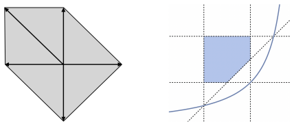
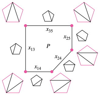
[Example 2.8] The sentence “The right part of Figure 1 shows a three-dimensional ABHY associahedron” is inconsistent with the figure as described: the right panel of Figure 1 is the two-dimensional polypol from Example 1.10. The intended reference appears to be to Figure 7 or to another panel; please correct it.
[Exercise 1] The word “invidual” should be “individual.”
[Definition 3.9 and Theorem 3.12] The symbol P is used both for the polypol and for the semi-algebraic set, e.g., in “a quasi-regular rational polypol P = (Y•, v•) with semi-algebraic set P”. Using a different letter for the region, such as X_≥0 or S, would avoid confusion.
[Example 2.13] The displayed substitutions for the universal adjoint are incomplete: after listing x13 = y1 + y0, x14 = y2 + y0, x24 = −y1 + y2 + y0, the remaining substitutions are omitted. Since this is meant as a check, the full list should be given or a reference to [22] supplied.

Circularity Check

0 steps flagged · score 0.0 of 10

No significant circularity: the notes are expository, the central theorems carry independent proofs, and the one self-identified interpretive step is disclosed rather than hidden.

full rationale

This paper is explicitly a set of lecture notes: the abstract states that 'the text is a collection of known results.' The central polytope result, Theorem 2.2, is proven by induction on dimension using explicit residue computations, with the Hodge-theoretic identification (Definition 1.13) imported from the external work of Brown and Dupont [9]; that work is not by the present author, and the notes quote specific propositions ([9, Props. 1.15, 2.14, 2.15, 3.26]) as independent support. Theorem 2.5 is explicitly referred to [2, Section 7.4], an external source. The main polypol theorem, Theorem 3.12, is quoted from [15] and accompanied by a self-contained proof sketch; although the present author is a co-author of [15], the cited theorem is a published external result with an independent proof, so this is provenance rather than a circular reduction. Proposition 2.11 invokes [22, Theorem 3.10] from the author's own work, but that theorem is an independent mathematical statement used for a peripheral adjoint-polynomial fact, not a renamed version of the conclusion being derived. The one genuinely delicate step, Definition 1.13, is explicitly introduced as 'inspired by (but not explicitly stated in) [9]', and the paper openly states that Definitions 1.4 and 1.13 are not equivalent and that not all genus-zero pairs should necessarily be called positive geometries. This transparency, together with the external citations, means no claim in the paper is equivalent to its inputs by construction. No fitted parameter is renamed as a prediction, and no equation is shown to reduce to a prior definition in a circular way. The result is a faithful survey with self-citations used only as references to independent prior work, so the circularity score is 0.

Assumptions & free parameters 1 free parameters · 4 assumptions · 0 invented entities

The notes introduce no new entities. The only normalization freedom is the global scalar alpha in equation (9), fixed by the residue condition rather than fit to data. All load-bearing mathematical input is inherited from [2], [9], and [15]. The active assumptions are the axiomatic framework of positive geometry and the specific genus-zero and adjoint results quoted from the literature.

free parameters (1)

Normalization constant alpha in polypol canonical form (equation 9) = Not numerically fixed; chosen so iterated residues at vertices are +/-1
Appears in Theorem 3.12. The canonical form is determined up to a global scalar, and alpha is fixed by the residue normalization condition. This is a gauge choice, not a parameter fitted to data.

assumptions (4)

domain assumption Existence and uniqueness of canonical forms satisfying the recursive residue axioms of Definition 1.4.
The entire framework assumes the recursive residue conditions single out a unique rational d-form. This is the positive geometry definition from [2], taken as a starting point rather than proved.
domain assumption The Brown-Dupont canonical map from relative homology to logarithmic forms exists for genus-zero pairs and has the residue and uniqueness properties stated in [9, Propositions 1.15, 2.14, and 2.15].
Used in Definition 1.13, the proof of Theorem 2.2, and Proposition 3.14 to identify canonical forms with logarithmic forms. The statements are cited, not proved in the notes.
domain assumption The pairs (P^d, Y_P) for polytopes and (Y_i, Z_i) for boundary curves have genus zero.
Invoked via [9, Proposition 3.26 and Section 3.3.2] in the proofs of Theorem 2.2 and Proposition 3.14. Without this property, the Hodge-theoretic identification fails.
domain assumption A nodal rational polypol has a unique adjoint curve, not containing any boundary curve or vertex.
Quoted as [15, Theorem 2.1] and used in Theorem 3.12 to fix the zero locus of the canonical form. The notes note that uniqueness can fail for non-rational boundary curves.

how reviews work

0 comments

Cite this review

Pith. "Pith review of Positive Geometry of Polytopes and Polypols." pith.science (2026). https://pith.science/paper/76PNXPTR

@misc{pith2026250605510,
  author       = {Pith},
  title        = {Pith review of: Positive Geometry of Polytopes and Polypols},
  year         = {2026},
  howpublished = {\url{https://pith.science/paper/76PNXPTR}},
  note         = {Machine review of arXiv:2506.05510}
}

read the original abstract

These are lecture notes supporting a minicourse taught at the Summer School in Total Positivity and Quantum Field Theory at CMSA Harvard in June 2025. We give an introduction to positive geometries and their canonical forms. We present the original definition by Arkani-Hamed, Bai and Lam, and a more recent definition suggested by work of Brown and Dupont. We compute canonical forms of convex polytopes and of quasi-regular polypols, which are nonlinear generalizations of polygons in the plane. The text is a collection of known results. It contains many examples and a list of exercises.

Figures

Figures reproduced from arXiv: 2506.05510 by the authors.

**Figure 2.** A positive geometry bounded by a parabola and a cuspidal cubic. [PITH_FULL_IMAGE:figures/full_fig_p006_2.png] view at source ↗

**Figure 3.** A positive geometry after blowing up a node. [PITH_FULL_IMAGE:figures/full_fig_p007_3.png] view at source ↗

Figures from the paper (6 more)

**Figure 4.** Figure 4: Two polytopes of dimension d = 2 (left) and d = 3 (right). Taken from [22]. [19]. For positive geometries in the wonderful compactification X of a hyperplane arrangement complement, see [8]. Lam discusses the positive geometry of the moduli space X = M0,n in [18]. Fina…

**Figure 5.** Figure 5: Left: the dual polygon of the pentagon P in Example 2.1. Right: the adjoint curve of P. Both figures are taken from [22]. of U ′ are u ′ F for F ∈ F(F1). The matrix U ′ is a submatrix of U satisfying | detU ′ v | = | detUv| for each v ∈ V(F1) ⊂ V(P). Here U ′ v is a (d…

**Figure 6.** Figure 6: The 2-dimensional associahedron [PITH_FULL_IMAGE:figures/full_fig_p013_6.png]

**Figure 7.** Figure 7: The amplitude as a sum over the 14 vertices of the 3D associahedron. [PITH_FULL_IMAGE:figures/full_fig_p013_7.png]

**Figure 8.** Figure 8: A quasiregular polypol with r = 4 and n = 8. The importance of Theorem 3.6 in constructing positive geometries in the sense of Definition 1.4 from polypols is explained intuitively as follows. We will soon associate a semialgebraic set P to P whose algebraic boundary…

**Figure 9.** Figure 9: A non-convex quadrilateral is a quasi-regular polypol. [PITH_FULL_IMAGE:figures/full_fig_p021_9.png]

Discussion (0). Sign in to comment.

Forward citations

Cited by 1 Pith paper

Reviewed papers in the Pith corpus that reference this work. Sorted by Pith novelty score. Full citation record

All Tree-Level Massive Cosmological Correlators via Spectral Gluing
hep-th 2026-07 conditional novelty 7.0 of 10

Tree-level massive de Sitter correlators are constructed by gluing Lauricella-type vertex functions according to graph combinatorics, and the hypergeometric content collapses to rational functions once the dynamical p...

Reference graph

Works this paper leans on

24 extracted references · 14 canonical work pages · cited by 1 Pith paper

[15]

K. Kohn, R. Piene, K. Ranestad, F. Rydell, B. Shapiro, R. Sinn, M.-Ş. Sorea, and S. Telen. Adjoints and canonical forms of polypols.Documenta Mathematica, 30(2):275–346, 2025

work page 2025
[2]

Arkani-Hamed, Y

N. Arkani-Hamed, Y. Bai, and T. Lam. Positive geometries and canonical forms.Journal of High Energy Physics, 2017(11):1–124, 2017

work page 2017
[9]

Brown and C

F. Brown and C. Dupont. Positive geometries and canonical forms via mixed Hodge theory. arXiv:2501.03202, 2025

arXiv 2025
[16]

Kohn and K

K. Kohn and K. Ranestad. Projective geometry of Wachspress coordinates.Foundations of Computa- tional Mathematics, 20(5):1135–1173, 2020

work page 2020
[22]

S. Telen. Toric amplitudes and universal adjoints.arXiv:2504.00897, 2025

arXiv 2025
[1]

Arkani-Hamed, Y

N. Arkani-Hamed, Y. Bai, S. He, and G. Yan. Scattering forms and the positive geometry of kinematics, color and the worldsheet.Journal of High Energy Physics, 2018(5):1–78, 2018

work page 2018
[3]

Arkani-Hamed, P

N. Arkani-Hamed, P. Benincasa, and A. Postnikov. Cosmological polytopes and the wavefunction of the universe.arXiv:1709.02813, 2017

arXiv 2017
[4]

Arkani-Hamed, C

N. Arkani-Hamed, C. Figueiredo, and F. Vazão. Cosmohedra.arXiv:2412.19881, 2024

arXiv 2024

Show all 24 references

[5]

Arkani-Hamed, H

N. Arkani-Hamed, H. Frost, G. Salvatori, P.-G. Plamondon, and H. Thomas. All loop scattering as a counting problem.arXiv:2309.15913, 2023

2023 arXiv
[6]

Arkani-Hamed, H

N. Arkani-Hamed, H. Frost, G. Salvatori, P.-G. Plamondon, and H. Thomas. All loop scattering for all multiplicity.arXiv:2311.09284, 2023

2023 arXiv
[7]

Arkani-Hamed and J

N. Arkani-Hamed and J. Trnka. The amplituhedron.Journal of High Energy Physics, 2014(10):1–33, 2014

2014
[8]

Brauner, C

S. Brauner, C. Eur, E. Pratt, and R. Vlad. Wondertopes.arXiv:2403.04610, 2024

2024
[10]

S. De, D. Pavlov, M. Spradlin, and A. Volovich. From Feynman diagrams to the amplituhedron: a gentle review.Le Matematiche, 80(1):233–254, 2025

2025
[11]

Early, A

N. Early, A. Geiger, M. Panizzut, B. Sturmfels, and C. H. Yun. Positive del Pezzo geometry.Annales de l’Institut Henri Poincaré D, To appear:To appear, 2023

2023
[12]

B. Eden, P. Heslop, and L. Mason. The correlahedron.Journal of High Energy Physics, 2017(9):1–42, 2017

2017
[13]

C. Gaetz. Canonical forms of polytopes from adjoints.arXiv:2504.07272, 2025

2025 arXiv
[14]

Hartshorne.Algebraic geometry, volume 52

R. Hartshorne.Algebraic geometry, volume 52. Springer Science & Business Media, 2013

2013
[17]

T. Lam. An invitation to positive geometries.Open Problems in Algebraic Combinatorics, 110:159–180, 2024

2024
[18]

T. Lam. Moduli spaces in positive geometry.Le Matematiche, 80(1):17–101, 2025

2025
[19]

Pavlov and K

D. Pavlov and K. Ranestad. Positive polytopes with few facets in the Grassmannian.arXiv:2503.01652, 2025

2025
[20]

Ranestad, R

K. Ranestad, R. Sinn, and S. Telen. Adjoints and canonical forms of tree amplituhedra.Mathematica Scandinavica, 130(2):433–466, 2024

2024
[21]

Ranestad, B

K. Ranestad, B. Sturmfels, and S. Telen. Logarithmic discriminants of hyperplane arrangements.Le Matematiche, 80(1):3–16, 2025

2025
[23]

E. L. Wachspress.A Rational Finite Element Basis. Academic Press, New York, 1975

1975
[24]

J. Warren. Barycentric coordinates for convex polytopes.Advances in Computational Mathematics, 6(1):97–108, 1996. Author’s address:Simon Telen, MPI-MiS Leipzigsimon.telen@mis.mpg.de 22

1996

Pith tools

Reviewed August 7, 2026 · model on record in the stance chip above.

[1] [15]

K. Kohn, R. Piene, K. Ranestad, F. Rydell, B. Shapiro, R. Sinn, M.-Ş. Sorea, and S. Telen. Adjoints and canonical forms of polypols.Documenta Mathematica, 30(2):275–346, 2025

work page 2025

[2] [2]

Arkani-Hamed, Y

N. Arkani-Hamed, Y. Bai, and T. Lam. Positive geometries and canonical forms.Journal of High Energy Physics, 2017(11):1–124, 2017

work page 2017

[3] [9]

Brown and C

F. Brown and C. Dupont. Positive geometries and canonical forms via mixed Hodge theory. arXiv:2501.03202, 2025

arXiv 2025

[4] [16]

Kohn and K

K. Kohn and K. Ranestad. Projective geometry of Wachspress coordinates.Foundations of Computa- tional Mathematics, 20(5):1135–1173, 2020

work page 2020

[5] [22]

S. Telen. Toric amplitudes and universal adjoints.arXiv:2504.00897, 2025

arXiv 2025

[6] [1]

Arkani-Hamed, Y

N. Arkani-Hamed, Y. Bai, S. He, and G. Yan. Scattering forms and the positive geometry of kinematics, color and the worldsheet.Journal of High Energy Physics, 2018(5):1–78, 2018

work page 2018

[7] [3]

Arkani-Hamed, P

N. Arkani-Hamed, P. Benincasa, and A. Postnikov. Cosmological polytopes and the wavefunction of the universe.arXiv:1709.02813, 2017

arXiv 2017

[8] [4]

Arkani-Hamed, C

N. Arkani-Hamed, C. Figueiredo, and F. Vazão. Cosmohedra.arXiv:2412.19881, 2024

arXiv 2024