Beating joint quantum estimation limits with stepwise multiparameter metrology

Abolfazl Bayat; Chiranjib Mukhopadhyay; Matteo G.A. Paris; Victor Montenegro

REVIEW 4 major objections 4 minor 77 references

Beating joint quantum estimation limits with stepwise multiparameter metrology

T0 review · 4 major / 4 minor · reviewed 2026-08-07 · deepseek-v4-flash

Challenge this review Re-run · record.json Download PDF Read on arXiv ↗

Pith's one-line read Stepwise estimation—splitting the measurement budget into two sequential single-parameter rounds—beats the joint-estimation quantum bound whenever the two-parameter quantum Fisher information matrix is nearly singular, and restores L^-1.8…

desk verdict Sensible idea undermined by a missing error-propagation term in the central bound; the paper is worth reviewing but not publishable as is. read the letter →

arxiv 2506.06075 v1 pith:BHYL6RZI submitted 2025-06-06 quant-ph

Chiranjib Mukhopadhyay , Abolfazl Bayat , Victor Montenegro , Matteo G.A. Paris This is my paper

classification quant-ph

keywords stepwiseestimationmultiparameterquantummetrologyFisherinformationmatrixjointBayesiansensingmany-bodycriticalityLandau-ZenermodelmixedIsing

verification ladder T0 review T1 audit T2 compute T3 formal

The pith

A machine-rendered reading of the paper's core claim, the machinery that carries it, and where it could break.

The reading

The paper proposes stepwise estimation (SE) for two-parameter quantum metrology: spend m1 of M measurement rounds estimating one parameter, then use the remaining m2 rounds to estimate the second parameter at the first estimate. It proves a sufficient condition, $Q12^{2}$/(Q11Q22) > 2√2−2 ≈ 0.828, under which the SE precision bound is strictly below the joint estimation (JE) bound, meaning SE is guaranteed to win when the quantum Fisher information matrix is nearly singular. In a mixed Ising many-body probe near the first-order critical point, the SE bound decreases as $L^{-1}$.8 while the JE bound only as $L^{-1}$, so the quantum-enhanced scaling that parameter correlations destroy for joint estimation is recovered. Bayesian simulations with fixed, nonadaptive measurements on qubit, three-level Landau-Zener, and mixed Ising probes reach or approach the SE bound and beat the JE bound. The paper's central claim is that incompatible measurements and near-singular Fisher matrices need not be a barrier: sequential single-parameter strategies can outperform the ultimate but generally unreachable joint-estimation limit.

What carries the argument

The central object is the two-parameter quantum Fisher information matrix (QFIM), whose inverse sets the Cramér-Rao lower bound on the covariance of unbiased estimators. The key identities are the joint bound µ = Tr[$Q^{{-1}}$] and the stepwise bound ˜μ = min_γ [ (Q22/(Q11Q22−$Q12^{2}$))/γ + 1/((1−γ)Q22) ] (or the analogous expression with the order reversed), where γ = m1/M is the measurement-budget split. The off-diagonal correlation r = $Q12^{2}$/(Q11Q22) measures how close the QFIM is to singular; the proof of the sufficiency condition optimizes over γ and shows joint estimation can beat stepwise for all γ only when r ≤ 2√2−2. The many-body scaling result uses QFIM elements computed in the mixed Ising ground state, where criticality makes individual elements large but the matrix nearly singular, so joint estimation loses the quantum enhancement while stepwise estimation does not.

What would settle it

Simulate two-step estimation with a first-stage Gaussian error of variance $σ1^{2}$ and a second stage whose Q22 is evaluated at the estimated parameter, including the propagation term (∂Q22/∂λ1)^2 $σ1^{2}$/(m2 $Q22^{2}$) in the total variance; if at parameters satisfying r > 0.828 the corrected stepwise total exceeds the joint bound µ/M, the central claim fails. At the mixed Ising point (1.9, 0.28), the SE variance must scale as $L^{-1}$.8, not $L^{-1}$.

Watch

Extended reading notes

Core claim

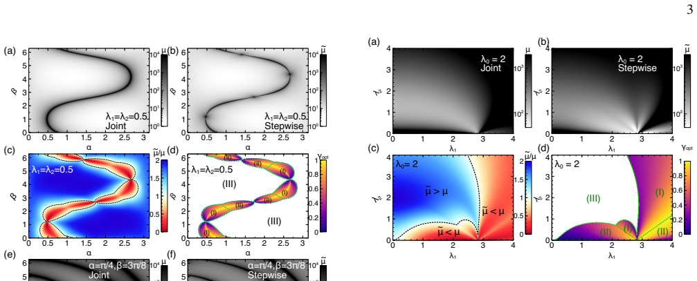
For any two-parameter estimation problem, if the off-diagonal correlation of the quantum Fisher information matrix satisfies r = $Q12^{2}$/(Q11Q22) ≥ 2√2−2 ≈ 0.828, the stepwise estimation bound is strictly lower than the joint estimation bound: the optimal SE bound, minimized over how the M rounds are split, falls below Tr[$Q^{{-1}}$]/M. Because r = 1 for a singular QFIM, the criterion selects models whose QFIM is close to singular, precisely the regime where joint estimation fails. In the mixed Ising ground state near the first-order critical point at (1.9, 0.28), the SE bound scales as $L^{-1}$.8 whereas the JE bound scales only as $L^{-1}$, restoring the quantum-enhanced sensitivity that near-singular parameter correlations remove from joint estimation. The paper also states a complementary result: for D-invariant models with nearly diagonal QFIM, the saturable Holevo Cramér-Rao bound for joint estimation always beats any stepwise strategy, so the SE advantage is tied to strong parameter correlation. Concrete Bayesian implementations using fixed measurement bases confirm that the SE advantage is realizable, not merely formal.

Load-bearing premise

The stepwise bound treats the first-stage estimate as exact when computing the second-stage Fisher information, so the claimed advantage assumes no error from the first stage leaks into the second; if it does, the total error can be larger than the bound says.

Editorial extensions

If this is right

In any two-parameter quantum model with QFIM correlation r > 0.828, the standard joint-estimation precision bound is not the full story: a sequential strategy is guaranteed a lower error bound.
Near-singular QFIMs, which arise naturally in many-body impurity probes, optical spatial-modulation sensing, and private sensor networks, are precisely where stepwise estimation should be used instead of joint estimation.
In many-body critical probes such as the mixed Ising model near the first-order transition, stepwise estimation restores quantum-enhanced scaling: L^-1.8 instead of the L^-1 shot-noise scaling that joint estimation yields.
The Bayesian demonstrations indicate the advantage is practically accessible with fixed, simple measurement bases, so the benefit does not require adaptive feedback or complicated joint measurements.
The optimal budget split approaches γ ≈ 0.5 for large system sizes, so an approximately equal division of measurement rounds between the two parameters is near-optimal in the scalable regime.

Reading between the lines

Editorial extensions of the paper, not claims the author makes directly.

The threshold 2√2−2 was derived for equal weighting of the two parameters (W = I2); if one parameter matters more than the other, the threshold would shift, and mapping how the threshold depends on the weight matrix is a natural extension of the paper's result.
The stepwise bound assumes no error propagation from the first-stage estimate to the second stage; a more detailed two-step model including the propagation term (∂Q22/∂λ1)^2 σ1^2/(m2 Q22^2) could shrink the practical advantage region, so testing this is an open problem.
The Bayesian comparison uses posterior variance against a frequentist Cramér-Rao bound without explicitly separating prior information from estimator bias; a fully Bayesian risk bound such as the van Trees inequality might give a fairer benchmark for the numerical demonstrations.
Theorem 2's statement that joint estimation wins near diagonal QFIMs is proven for D-invariant models; whether some non-D-invariant models admit stepwise advantages even near diagonal QFIMs remains an open question.

Share X Bluesky LinkedIn Reddit HN

Editorial analysis

A structured set of objections, weighed in public.

Desk editor's note, referee report, and a circularity audit.

Desk Editor's Note

read the letter

The stepwise idea is worth a look: splitting multiparameter estimation into sequential single-parameter steps is a natural way to dodge measurement incompatibility, and the paper works through several concrete models with a Bayesian implementation. That part is solid. But the analytical engine, Eq. (3) (and Eq. S14), is not a valid lower bound for the proposed two-stage procedure. The second term, 1/(m2 Q22), is the single-parameter QCRB for lambda2 only when lambda1 is known exactly. In the actual protocol lambda1 is replaced by a random estimate whose error is O(1/sqrt(m1)). For any second-stage measurement whose distribution depends on lambda1, that error propagates into the lambda2 estimate and contributes a variance term of order 1/m1, the same order as the terms kept in Eq. (3). The stress-test Gaussian model makes this concrete: with Q = [[1+c^2, c],[c,1]] and an equal split, the actual two-step variance sum is 2(2+c^2)/M, while Eq. (3) gives 4/M; for c^2=5 the paper's condition predicts SE wins, but the actual stepwise estimator is worse than the JE bound. So the sufficiency condition (6) and the L^-1.8 scaling claim compare an unattainable SE bound against the JE bound; they do not establish that any stepwise protocol beats joint estimation.

What the paper does well: it is clearly written, the sequential protocol is well defined, and the worked examples — qubit, Landau-Zener, mixed Ising, coherent-state probe — give a concrete feel for where near-singular QFIMs arise. The Bayesian demonstrations are useful as existence proofs that some sequential protocol can perform well, but they compare Bayesian posterior variance against frequentist QCRBs, and they are preselected in regions where the (flawed) bound predicts an advantage. The necessary condition for the Holevo bound (Theorem 2) is a separate result and may survive, but it does not fix the sufficiency condition.

Bottom line: the core claim is not supported as written. The fix isn't trivial — you need to either include the propagation term in the SE bound (and then the condition will look different), or identify special cases where the second-stage measurement is insensitive to the first parameter, or prove a valid bound for a specific adaptive estimator. If the authors can do that, the idea could have legs. As it stands, this is a well-posed but unproven conjecture.

Recommendation: I'd send it to peer review — the topic matters and the flaw is instructive — but with a clear expectation that the main theorem must be reworked. It should not be published in its current form.

Referee Report

4 major / 4 minor

Summary. The paper proposes a stepwise estimation (SE) protocol for two-parameter quantum metrology: allocate m1 measurement rounds to estimate one parameter, then feed the resulting point estimate into a single-parameter estimation of the second parameter over m2 rounds. It derives a precision bound in Eq. (3) and a sufficient condition Eq. (6) under which this bound lies below the joint-estimation (JE) bound. The authors illustrate the claimed advantage for a qubit probe, a three-level Landau-Zener probe, a coherent-state Gaussian probe, and a many-body mixed Ising model, including Bayesian simulations. The main advertised results are that SE can beat JE near singular QFIMs and can restore quantum-enhanced scaling (claimed L^{-1.8}) near a first-order critical point where joint estimation scales only as L^{-1}.

Significance. If the central bound were valid, the paper would address two recognized problems in multiparameter quantum metrology: the non-attainability of the QFIM bound due to measurement incompatibility and the degradation of precision when the QFIM is near singular. The paper is explicit and offers several worked examples, including an analytic sufficiency condition and a discussion of the Holevo CRB in the supplemental material. However, the entire framework rests on Eq. (3), and that expression is not a valid lower bound for the two-stage protocol as described. The claimed sufficiency condition, the scaling comparison in Fig. 3(e), and the Bayesian demonstrations therefore do not establish that any stepwise procedure actually outperforms joint estimation. The idea is interesting and the examples are clearly presented, but the core technical claim needs a corrected derivation before the conclusions can be accepted.

major comments (4)

[Eq. (3) and SM Eq. (S14)] The right-hand side of Eq. (3) is not a lower bound on the variance sum of the two-stage procedure described in the text. The first term is a legitimate scalar Cramer-Rao bound for estimating lambda1 with lambda2 as a nuisance parameter. The second term, 1/(m2 Q22(lambda_est1, lambda2)), is the single-parameter QCRB for lambda2 only when lambda1 is known exactly. In the actual protocol lambda1 is replaced by the random estimator lambda_est1 whose variance is O(1/m1). Any estimator of lambda2 based on the second-stage data inherits an additional variance term of order 1/m1 whenever the second-stage outcome distribution depends on lambda1. Since m1 = gamma M, this propagation term is O(1/M), the same order as the terms retained in Eq. (3). A concrete Gaussian model with QFIM Q = [[1+c^2, c], [c, 1]], measurements x ~ N(lambda1,1) and y ~ N(c lambda1 + lambda2,1), and m1 = m2 = M/2 gives an actual stepwise variance sum of 2(2+c^2)/M, whereas Eq. (3) predicts 4/M. The omitted c^2 term is of the same order and is largest exactly in the strongly correlated regime where Eq. (6) is invoked.
[Theorem 1 and Eq. (6)] The sufficiency condition Q12^2/(Q11 Q22) > 2*sqrt(2)-2 is derived by optimizing the invalid bound in Eq. (3), so the theorem does not establish that any unbiased stepwise estimator outperforms joint estimation. The algebraic steps from Eq. (S16) to Eq. (S23) are internally consistent, but they manipulate an incorrect starting inequality. The supplemental discussion of the Holevo CRB does not repair this gap because the SE bounds mu' and mu'' used in Eqs. (S24)-(S31) are still based on the same unjustified additivity assumption.
[Fig. 3(e) and the L^{-1.8} scaling claim] The claimed restoration of quantum-enhanced scaling near the first-order critical point of the mixed Ising model compares the joint bound mu ~ L^{-1} with the stepwise bound mu_tilde ~ L^{-1.8}. Since mu_tilde is computed from Eq. (3), the comparison is between a generally unattainable JE bound and an unattainable, overly optimistic SE bound. A corrected two-stage bound that includes the first-stage error propagation could scale differently, particularly near a near-singular QFIM where the propagation term is enhanced. The statement that SE 'restores' the quantum advantage is therefore not supported by the presented calculations.
[Bayesian Implementation (Fig. 4 and SM 'Bayesian Scheme')] The Bayesian demonstration compares posterior variances against frequentist Cramer-Rao bounds without accounting for the contribution of the prior. Uniform priors with widths pi/5, 0.2, and 1 for the three examples are additional free inputs, and the true parameter values are preselected from the region where Eq. (6) holds. The observed posterior variances are not a test of the claimed SE bound: a Bayesian estimator with informative prior can appear to 'reach' a frequentist bound or even fall below it for reasons unrelated to the two-stage protocol. This undermines the third main result as a validation of the analytical claims.

minor comments (4)

[Eq. (4)] The weight matrix in Eq. (4) is written as W1=diag(0,1); it should be W2=diag(0,1) to match the notation introduced for the two ordering strategies.
[Introduction, Landau-Zener paragraph] The phrase 'gap-closing []' contains an empty citation placeholder; a reference to the gap-closing condition or to a relevant review should be inserted.
[SM Eq. (S33)] The Bayesian update formula writes lambda_est1 = sum over lambda1 of lambda1 p1(lambda1|x1), which is only valid for a discrete grid of parameter values; the continuous analogue should be stated for clarity, since the main text treats the parameters as continuous.
[Figure 4 captions] The captions for the right-hand panels state that 'Var x M' is plotted, but the text in the main body sometimes refers to 'sum of Bayesian variances multiplied by M'; the notation should be made consistent so the reader can identify which quantity is compared with mu and mu_tilde.

Circularity Check

0 steps flagged · score 0.0 of 10

No significant circularity: the central SE-vs-JE comparison is a direct algebraic consequence of the QFIM, not a self-imported conclusion.

full rationale

The derivation chain is self-contained. The stepwise bound in Eq. (3) is formed from the diagonal entries of Q^{-1} plus the single-parameter inverse QFI 1/Q22; the joint bound in Eq. (2) is Tr[Q^{-1}]/M. The sufficiency condition in Eq. (6) is obtained in the Supplemental Material by algebraically comparing Eqs. (S13) and (S14) and minimizing over the measurement budget γ; it does not use data, fitted parameters, or the paper's own conclusions as inputs. The many-body scaling comparison and Bayesian demonstrations use the same QFIM as input and check the derived bound's regime, which is a consistency check rather than a circular prediction. The cited Holevo and Suzuki bounds are external results, and the paper's self-citations appear only as background or review references, not as load-bearing justification for the main claim. The concern that Eq. (3) omits first-stage error propagation is a validity or attainability objection, not an instance of a quantity being defined in terms of the claimed output; no step in the derivation is equivalent to its input by construction.

Assumptions & free parameters 2 free parameters · 3 assumptions · 0 invented entities

The central derivation is a two-parameter Fisher-information analysis built on standard quantum estimation theory. No new particles or forces are postulated. The analytical results rely on asymptotic local estimation assumptions and, in the Holevo comparison, on D-invariance. The Bayesian demonstrations introduce hand-chosen priors and measurement budgets, which are not fitted to data but influence the numerical comparison.

free parameters (2)

Bayesian prior widths = qubit: π/5, three-level LZ: 0.2, mixed Ising: 1
Hand-chosen support widths for the uniform priors in the Bayesian simulations. They do not enter the analytical bound but influence the finite-M posterior variance and the comparison against the joint Cramér-Rao bound.
Measurement budget γ = 0.7 (qubit), 0.3 (LZ), 0.5 (Ising)
Chosen close to the theoretically optimal split of measurement rounds for each example. It is a design choice for the demonstration, not a fit to data, but it affects the numerical results.

assumptions (3)

domain assumption The single-parameter quantum Cramér-Rao bound is saturable in the asymptotic limit.
Used throughout to convert QFIM elements into achievable variance bounds for each step of the stepwise scheme. This is standard in the field but an assumption about asymptotic behavior.
domain assumption The replacement Q22(λest_1, λ2) ≈ Q22(λ1, λ2) in the asymptotic limit is legitimate.
Invoked after Eq. (5) in the main text and in the SM. It requires consistency of the first-step estimator and smoothness of the QFIM, and it ignores the propagation of the first-step error into the second-step model.
domain assumption D-invariant models are used for the Holevo-bound comparison in Theorem 2 and Eq. (S31).
The necessary condition for beating the Holevo bound applies only to D-invariant probes. The paper does not verify D-invariance for the qubit, LZ, and Ising examples, so the Holevo-related statements are conditional.

how reviews work

0 comments

Cite this review

Pith. "Pith review of Beating joint quantum estimation limits with stepwise multiparameter metrology." pith.science (2026). https://pith.science/paper/BHYL6RZI

@misc{pith2026250606075,
  author       = {Pith},
  title        = {Pith review of: Beating joint quantum estimation limits with stepwise multiparameter metrology},
  year         = {2026},
  howpublished = {\url{https://pith.science/paper/BHYL6RZI}},
  note         = {Machine review of arXiv:2506.06075}
}

read the original abstract

Conventional multiparameter quantum sensing relies on joint estimation, but this approach faces two key limitations: theoretical bounds may be unattainable due to measurement incompatibility, and sensing may fail due to parameter interdependencies. We propose stepwise estimation and identify regimes where it outperforms joint estimation. For multiple quantum sensors, this scheme achieves far lower error bounds than joint estimation. With many-body probes, stepwise sensing retains a quantum-enhanced scaling advantage often lost in joint estimation due to parameter correlations. We demonstrate its concrete advantages through Bayesian implementations across diverse examples.

Figures

Figures reproduced from arXiv: 2506.06075 by the authors.

**Figure 1.** FIG. 1. Qubit probe estimating ( [PITH_FULL_IMAGE:figures/full_fig_p003_1.png] view at source ↗

**Figure 3.** FIG. 3. Mixed Ising probe estimating ( [PITH_FULL_IMAGE:figures/full_fig_p004_3.png] view at source ↗

Figures from the paper (1 more)

**Figure 4.** Figure 4: FIG. 4. Bayesian SE for (a)-(b) qubit probe estimating ( [PITH_FULL_IMAGE:figures/full_fig_p004_4.png]

Discussion (0). Sign in to comment.

Reference graph

Works this paper leans on

77 extracted references · 67 canonical work pages

[1]

Giovannetti, S

V . Giovannetti, S. Lloyd, and L. Maccone, Physical review let- ters 96, 010401 (2006)

2006
[2]

Giovannetti, S

V . Giovannetti, S. Lloyd, and L. Maccone, Nature photonics 5, 222 (2011)

2011
[3]

Xiang and G.-C

G.-Y . Xiang and G.-C. Guo, Chinese Physics B 22, 110601 (2013)

work page 2013
[4]

M. A. Taylor and W. P. Bowen, Physics Reports 615, 1 (2016)

work page 2016
[5]

Tóth and I

G. Tóth and I. Apellaniz, Journal of Physics A: Mathematical and Theoretical 47, 424006 (2014)

work page 2014
[6]

C. L. Degen, F. Reinhard, and P. Cappellaro, Reviews of Mod- ern Physics 89, 035002 (2017)

work page 2017
[7]

Polino, M

E. Polino, M. Valeri, N. Spagnolo, and F. Sciarrino, A VS Quan- tum Science 2 (2020)

work page 2020
[8]

DeMille, N

D. DeMille, N. R. Hutzler, A. M. Rey, and T. Zelevinsky, Na- ture Physics 20, 741 (2024)

work page 2024

Show all 77 references

[9]

Mishra and A

U. Mishra and A. Bayat, Physical Review Letters 127, 080504 (2021)

2021
[10]

Montenegro, U

V . Montenegro, U. Mishra, and A. Bayat, Physical Review Let- ters 126, 200501 (2021)

2021
[11]

Mishra and A

U. Mishra and A. Bayat, Scientific Reports 12, 14760 (2022)

2022
[12]

C. D. Marciniak, T. Feldker, I. Pogorelov, R. Kaubruegger, D. V . Vasilyev, R. van Bijnen, P. Schindler, P. Zoller, R. Blatt, and T. Monz, Nature 603, 604 (2022)

2022
[13]

X. He, R. Yousefjani, and A. Bayat, Physical Review Letters 131, 010801 (2023)

2023
[14]

Mukhopadhyay, V

C. Mukhopadhyay, V . Montenegro, and A. Bayat, Journal of Physics A: Mathematical and Theoretical 58, 063001 (2025)

2025
[15]

Mukhopadhyay, M

C. Mukhopadhyay, M. G. Paris, and A. Bayat, arXiv preprint arXiv:2410.12050 (2024)

2024 arXiv
[16]

Qvarfort, A

S. Qvarfort, A. Serafini, P. F. Barker, and S. Bose, Nature com- munications 9, 3690 (2018)

2018
[17]

Montenegro, Phys

V . Montenegro, Phys. Rev. Res.7, 013016 (2025)

2025
[18]

H. Y . Kwon, H. Yoon, C. Lee, G. Chen, K. Liu, A. Schmid, Y . Wu, J. Choi, and C. Won, Science advances 6, eabb0872 (2020)

2020
[19]

Campos Venuti and P

L. Campos Venuti and P. Zanardi, Physical Review Letters 99, 095701 (2007)

2007
[20]

Zanardi, M

P. Zanardi, M. G. Paris, and L. Campos Venuti, Physical Re- view A—Atomic, Molecular, and Optical Physics 78, 042105 (2008)

2008
[21]

Shabani, M

A. Shabani, M. Mohseni, S. Lloyd, R. L. Kosut, and H. Rabitz, Physical Review A—Atomic, Molecular, and Optical Physics 84, 012107 (2011)

2011
[22]

Dooley, PRX Quantum 2, 020330 (2021)

S. Dooley, PRX Quantum 2, 020330 (2021)

2021
[23]

Sarkar, C

S. Sarkar, C. Mukhopadhyay, A. Alase, and A. Bayat, Physical Review Letters 129, 090503 (2022)

2022
[24]

Montenegro, M

V . Montenegro, M. G. Genoni, A. Bayat, and M. G. A. Paris, Phys. Rev. Res. 4, 033036 (2022)

2022
[25]

Mukhopadhyay and A

C. Mukhopadhyay and A. Bayat, Physical Review Letters 133, 120601 (2024)

2024
[26]

Sahoo, U

A. Sahoo, U. Mishra, and D. Rakshit, Physical Review A 109, L030601 (2024)

2024
[27]

Ye and P

J. Ye and P. Zoller, Physical Review Letters 132, 190001 (2024)

2024
[28]

Zhang, P

T. Zhang, P. Xu, J. Hu, and X. Qiu, New Journal of Physics (2025)

2025
[29]

Burgarth and A

D. Burgarth and A. Ajoy, Physical Review Letters 119, 030402 (2017)

2017
[30]

Demkowicz-Dobrza ´nski, W

R. Demkowicz-Dobrza ´nski, W. Górecki, and M. Gu¸ t˘a, Journal of Physics A: Mathematical and Theoretical53, 363001 (2020)

2020
[31]

Szczykulska, T

M. Szczykulska, T. Baumgratz, and A. Datta, Advances in Physics: X 1, 621 (2016)

2016
[32]

J. Liu, H. Yuan, X.-M. Lu, and X. Wang, Journal of Physics A: Mathematical and Theoretical 53, 023001 (2020)

2020
[33]

J. J. Meyer, Quantum 5, 539 (2021)

2021
[34]

Petz and C

D. Petz and C. Ghinea, in Quantum probability and related top- ics (World Scientific, 2011) pp. 261–281

2011
[35]

Mihailescu, S

G. Mihailescu, S. Campbell, and K. Gietka, Physical Review A 111, 052621 (2025)

2025
[36]

A. Z. Goldberg, J. L. Romero, Á. S. Sanz, and L. L. Sánchez-Soto, International Journal of Quantum Information 19, 2140004 (2021)

2021
[37]

Razavian, M

S. Razavian, M. G. Paris, and M. G. Genoni, Entropy 22, 1197 (2020)

2020
[38]

Frigerio and M

M. Frigerio and M. G. Paris, arXiv preprint arXiv:2410.02989 (2024)

2024 arXiv
[39]

Y . Yang, V . Montenegro, and A. Bayat, arXiv preprint arXiv:2501.02784 (2025)

2025
[40]

Mihailescu, S

G. Mihailescu, S. Sarkar, A. Bayat, S. Campbell, and A. K. Mitchell, arXiv preprint arXiv:2503.05483 (2025). 6

2025
[41]

He and M

J. He and M. G. Paris, arXiv preprint arXiv:2503.08235 (2025)

2025 arXiv
[42]

Mihailescu, A

G. Mihailescu, A. Bayat, S. Campbell, and A. K. Mitchell, Quantum Science and Technology 9, 035033 (2024)

2024
[43]

Candeloro, Z

A. Candeloro, Z. Pazhotan, and M. G. Paris, Quantum Science and Technology 9, 045045 (2024)

2024
[44]

C. Peng, K. Zheng, R.-B. Jin, C. Ding, and X. Hao, Journal of Applied Physics 133, 163102 (2023)

2023
[45]

Hassani, S

M. Hassani, S. Scheiner, M. G. A. Paris, and D. Markham, Phys. Rev. Lett. 134, 030802 (2025)

2025
[46]

S. Ragy, M. Jarzyna, and R. Demkowicz-Dobrza ´nski, Physical Review A 94, 052108 (2016)

2016
[47]

Carollo, B

A. Carollo, B. Spagnolo, A. A. Dubkov, and D. Valenti, Journal of Statistical Mechanics: Theory and Experiment 2019, 094010 (2019)

2019
[48]

Belliardo and V

F. Belliardo and V . Giovannetti, New Journal of Physics 23, 063055 (2021)

2021
[49]

B. Xia, J. Huang, H. Li, H. Wang, and G. Zeng, Nature Com- munications 14, 1021 (2023)

2023
[50]

Albarelli and R

F. Albarelli and R. Demkowicz-Dobrza´nski, Physical Review X 12, 011039 (2022)

2022
[51]

H. Chen, Y . Chen, and H. Yuan, Physical Review A 105, 062442 (2022)

2022
[52]

Gessner, L

M. Gessner, L. Pezzè, and A. Smerzi, Physical review letters 121, 130503 (2018)

2018
[53]

T. J. Proctor, P. A. Knott, and J. A. Dunningham, Physical re- view letters 120, 080501 (2018)

2018
[54]

Nichols, P

R. Nichols, P. Liuzzo-Scorpo, P. A. Knott, and G. Adesso, Physical Review A 98, 012114 (2018)

2018
[55]

Gessner, A

M. Gessner, A. Smerzi, and L. Pezzè, Nature communications 11, 3817 (2020)

2020
[56]

A. Z. Goldberg, L. L. Sánchez-Soto, and H. Ferretti, Physical Review Letters 127, 110501 (2021)

2021
[57]

Albarelli, M

F. Albarelli, M. Barbieri, M. G. Genoni, and I. Gianani, Physics Letters A 384, 126311 (2020)

2020
[58]

J. J. Meyer, J. Borregaard, and J. Eisert, npj Quantum Informa- tion 7, 89 (2021)

2021
[59]

Rubio and J

J. Rubio and J. Dunningham, Physical Review A 101, 032114 (2020)

2020
[60]

Di Fresco, B

G. Di Fresco, B. Spagnolo, D. Valenti, and A. Carollo, SciPost Physics 13, 077 (2022)

2022
[61]

Cramér, Scandinavian Actuarial Journal 1946, 85 (1946)

H. Cramér, Scandinavian Actuarial Journal 1946, 85 (1946)

1946
[62]

C. R. Rao, in Breakthroughs in Statistics: F oundations and ba- sic theory (Springer, 1992) pp. 235–247

1992
[63]

A. S. Holevo, in Proceedings of the Third Japan—USSR Sym- posium on Probability Theory (Springer, 2006) pp. 194–222

2006
[64]

Albarelli, J

F. Albarelli, J. F. Friel, and A. Datta, Physical Review Letters 123, 200503 (2019)

2019
[65]

Suzuki, Journal of Mathematical Physics 57 (2016)

J. Suzuki, Journal of Mathematical Physics 57 (2016)

2016
[66]

Bressanini, M

G. Bressanini, M. G. Genoni, M. Kim, and M. G. Paris, arXiv preprint arXiv:2403.03919 (2024)

2024 arXiv
[67]

Chang, M

S. Chang, M. G. Genoni, and F. Albarelli, arXiv preprint arXiv:2504.17873 (2025)

2025 arXiv
[68]

Suzuki, arXiv preprint arXiv:1807.06990 (2018)

J. Suzuki, arXiv preprint arXiv:1807.06990 (2018)

2018 arXiv
[69]

Montenegro, C

V . Montenegro, C. Mukhopadhyay, R. Yousefjani, S. Sarkar, U. Mishra, M. G. Paris, and A. Bayat, arXiv preprint arXiv:2408.15323 (2024)

2024 arXiv
[70]

Carroll and F

C. Carroll and F. Hioe, Journal of Physics A: Mathematical and Theoretical 19, 1151 (1986)

1986
[71]

S. N. Shevchenko, S. Ashhab, and F. Nori, Physics Reports 492, 1 (2010)

2010
[72]

Band and Y

Y . Band and Y . Avishai, Physical Review A99, 032112 (2019)

2019
[73]

Bakmou and M

L. Bakmou and M. Daoud, Journal of Physics A: Mathematical and Theoretical 53, 385301 (2020). SUPPLEMENTAL MA TERIAL Brief Review of Multiparameter Quantum Estimation In the joint estimation (JE) setting, the precision bound for sum of variances of the two estimators ˆΛ1, ˆΛ2 ...

2020
[74]

That is, stepwise estimation is always guaranteed to succeed when Q12 Q11 ! Q12 Q22 ! ≥ 2 √ 2− 2≈ 0.828 (S23) This completes the proof of the theorem

Thus, in any problem where Q11Q22−Q2 12 Q11Q22 ≤ 3−2 √ 2 is where stepwise estimation will have a better result than joint estimation. That is, stepwise estimation is always guaranteed to succeed when Q12 Q11 ! Q12 Q22 ! ≥ 2 √ 2− 2≈ 0.828 (S23) This completes the proof of the ...
[75]

(S21) with equal weights

Notice that in the proof of the previous theorem, we implicitly assumedχ= 1 2 as we added up the two bounds in Eq. (S21) with equal weights. Now for QFIM close to diagonal, we can do the following perturbation expansions 1 Q11 = Q22 ∆ 1 + Q2 12 ∆  −1 ≈ Q22 ∆ ...
[76]

For example, for qubits, this can be a numerically simulated by a binary string randomly picked via binomial probabilities given by the true parameter

Estimatingλ1 – Let us assume the measurement result is x1. For example, for qubits, this can be a numerically simulated by a binary string randomly picked via binomial probabilities given by the true parameter. The posterior of the first parameter is then given by the Bayes ru...
[77]

Typically this measurement is performed in a di fferent basis than the first step

Estimatingλ2 – Armed with the Bayesian estimate of the first parameter, now we can update the prior p2 of the second parameter λ2 after another round of simulated measurements x2 given by another binary string randomly picked via binomial probabilities given by the true parame...

Pith tools

Reviewed August 7, 2026 · model on record in the stance chip above.

[1] [1]

Giovannetti, S

V . Giovannetti, S. Lloyd, and L. Maccone, Physical review let- ters 96, 010401 (2006)

2006

[2] [2]

Giovannetti, S

V . Giovannetti, S. Lloyd, and L. Maccone, Nature photonics 5, 222 (2011)

2011

[3] [3]

Xiang and G.-C

G.-Y . Xiang and G.-C. Guo, Chinese Physics B 22, 110601 (2013)

work page 2013

[4] [4]

M. A. Taylor and W. P. Bowen, Physics Reports 615, 1 (2016)

work page 2016

[5] [5]

Tóth and I

G. Tóth and I. Apellaniz, Journal of Physics A: Mathematical and Theoretical 47, 424006 (2014)

work page 2014

[6] [6]

C. L. Degen, F. Reinhard, and P. Cappellaro, Reviews of Mod- ern Physics 89, 035002 (2017)

work page 2017

[7] [7]

Polino, M

E. Polino, M. Valeri, N. Spagnolo, and F. Sciarrino, A VS Quan- tum Science 2 (2020)

work page 2020

[8] [8]

DeMille, N

D. DeMille, N. R. Hutzler, A. M. Rey, and T. Zelevinsky, Na- ture Physics 20, 741 (2024)

work page 2024