Magnetogenesis from Sawtooth Coupling: Gravitational Wave Probe of Reheating

Subhasis Maiti

REVIEW 3 major objections 5 minor 1 cited by

Magnetogenesis from Sawtooth Coupling: Gravitational Wave Probe of Reheating

T0 review · 3 major / 5 minor · reviewed 2026-08-07 · deepseek-v4-flash

Challenge this review Re-run · record.json Download PDF Read on arXiv ↗

Pith's one-line read A sawtooth coupling between the inflaton and the electromagnetic field, active through a long low-temperature reheating, can generate megaparsec-scale magnetic fields and a blue-tilted gravitational wave background that current and…

desk verdict Careful incremental model of sawtooth-coupling magnetogenesis with reheating EoS dependence, whose headline B0 window rests on a questionable adiabatic assumption for a subhorizon 1 Mpc mode. read the letter →

arxiv 2506.06183 v2 pith:QJOF2MOM submitted 2025-06-06 astro-ph.CO hep-ph

Subhasis Maiti This is my paper

classification astro-ph.COhep-ph

keywords primordialmagneticfieldsreheatingsecondarygravitationalwavessawtoothcouplingblue-tiltedspectrumpulsartimingarraysLISAmagnetogenesis

verification ladder T0 review T1 audit T2 compute T3 formal

The pith

A machine-rendered reading of the paper's core claim, the machinery that carries it, and where it could break.

The reading

This paper sets out to show that a single broken power-law coupling between the electromagnetic field and the inflaton can explain large-scale cosmic magnetism without the usual strong-coupling and backreaction problems. The coupling rises during inflation as $f(a)\propto a^n$, falls during reheating as $f(a)\propto a^{-m}$, and returns to $f=1$ at the end of reheating. The central claim is that a prolonged reheating with a low temperature in roughly $10^{-2}$ to $10^{2}$ GeV yields present-day magnetic fields at the megaparsec scale that satisfy observational bounds, even though the magnetic spectrum is strongly blue-tilted rather than scale-invariant. The same electromagnetic fields act as a gravitational wave source, producing a broken power-law, blue-tilted secondary background that could be seen by PTA experiments, LISA, DECIGO, or BBO. Because the peak frequency of this background is set by the end of reheating, the signal would be a direct probe of reheating temperature and equation of state.

What carries the argument

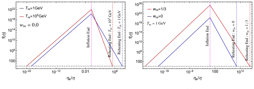
The load-bearing object is the sawtooth coupling function $f(a)$ defined in Eq. (8): it starts at unity at the beginning of inflation, grows as $(a/a_i)^n$ until inflation ends, shrinks as $(a_e/a_i)^n (a_e/a)^{-m}$ during reheating, and pins back to unity after reheating. In conformal time during reheating it behaves as $f(\eta)\propto (\eta_e/\eta)^{\alpha}$ with $\alpha=2n\beta/(1+3w_{\rm re})$, where $\beta=N_I/N_{\rm re}$. This functional form does three jobs at once: it keeps the effective electromagnetic coupling $e^2/f^2$ bounded above by its standard value, it keeps the produced electromagnetic energy density below the background for the allowed parameter range, and it sets the spectral index of the gauge-field mode function, which obeys a Bessel equation with effective potential $n(n+1)/\eta^2$ during inflation and $\alpha(\alpha+1)/\eta^2$ during reheating. The magnetic spectral energy density at the end of reheating inherits a blue tilt on super-horizon scales and a red tilt above $k_{\rm re}$, and the square of this spectrum sources the secondary gravitational waves.

What would settle it

Measure the spectral index of the stochastic gravitational wave background in the band $10^{-9}$--$10^{-7}$ Hz: the model predicts a strongly blue-tilted, broken power law with $\Omega_{\rm GW}\propto f^{2(4-2n)}$ on super-horizon scales, so a detected background that is red-tilted or has no break near the frequency set by $T_{\rm re}$ would rule out the parameter range that explains the 1 Mpc magnetic field. A sharper version is to check whether PTA datasets continue to prefer a red-tilted common-process signal with an energy-density index near $n_{\rm gw}\simeq 1.8$; if so, the secondary gravitational wave branch of this model is excluded for those parameters.

Watch

Extended reading notes

Core claim

The paper argues that the sawtooth coupling in Eq. (8) makes inflationary magnetogenesis viable at ordinary inflationary energy scales. With coupling parameters chosen so that the total electromagnetic energy density stays below the background at the end of reheating, the model produces present-day magnetic fields at 1 Mpc with strengths covering orders of magnitude, from about $10^{-26}$ G to $10^{-12}$ G, depending on $n$, $w_{\rm re}$, and $T_{\rm re}$. Because the coupling satisfies $f(\eta)\ge 1$ throughout, the effective gauge coupling never exceeds its standard value, which avoids the strong coupling problem. The magnetic field continues to grow during reheating, and its anisotropic stress sources tensor perturbations. The resulting gravitational wave energy density $\Omega_{\rm GW}h^2$ has a broken power-law shape, is blue-tilted on super-horizon scales as $\Omega_{\rm GW}\propto f^{2(4-2n)}$, and peaks near the mode that re-enters at the end of reheating, so it can fall within the sensitivity of PTA experiments, SKA, LISA, DECIGO, or BBO without requiring a very low inflationary scale.

Load-bearing premise

The paper assumes that some physical mechanism produces the broken power-law sawtooth coupling of Eq. (8) exactly as prescribed, and that after reheating megaparsec-scale modes redshift adiabatically with no magnetohydrodynamic effects; if either premise fails, the predicted field strengths and gravitational wave amplitudes do not follow.

Editorial extensions

If this is right

A strongly blue-tilted magnetic spectrum can satisfy present-day bounds on $B_0$ at 1 Mpc, provided reheating is prolonged and cold, with $T_{\rm re}$ roughly between $10^{-2}$ and $10^{2}$ GeV.
The secondary gravitational wave spectrum is a broken power law whose super-horizon branch scales as $\Omega_{\rm GW}\propto f^{2(4-2n)}$, making the signal distinguishable from the nearly scale-invariant primordial gravitational wave background.
For parameters that fit the magnetic bounds, the gravitational wave peak sits near the frequency $f_{\rm re}$ associated with the end of reheating, so detecting the peak frequency would measure the reheating temperature.
Generating observable secondary gravitational waves does not require a very low inflationary scale; values around $H_I\simeq 10^{-5}M_P$ are sufficient.
The model's blue-tilted nano-Hz signal can be compatible within $2\sigma$ with current PTA datasets such as NANOGrav and EPTA, rather than requiring a red-tilted interpretation.

Reading between the lines

Editorial extensions of the paper, not claims the author makes directly.

If the broken power-law secondary gravitational wave background is measured, the combination of spectral slope and peak frequency would jointly constrain the triple $(n, w_{\rm re}, T_{\rm re})$, an inversion the paper does not explicitly perform.
The model treats non-helical fields only; extending the sawtooth coupling to a helical or axion-like counterpart would predict circularly polarized gravitational waves and could be tested by future polarization-sensitive detectors.
Because the currently favored PTA common-process signal is red-tilted, the blue-tilted spectrum predicted here would likely need to be a subdominant component of the observed background; a direct measurement of the spectral index in the $10^{-9}$--$10^{-7}$ Hz band is a sharper test than the overall amplitude alone.
The sawtooth ansatz would become falsifiable from the microphysical side if no controlled field theory produces $f(a)\propto a^{-m}$ during reheating while restoring $f=1$ at the end.

Share X Bluesky LinkedIn Reddit HN

Editorial analysis

A structured set of objections, weighed in public.

Desk editor's note, referee report, and a circularity audit.

Desk Editor's Note

read the letter

Read this as an incremental but mostly careful model-building paper. The new piece is the systematic inclusion of the reheating equation of state and temperature in the sawtooth-coupling magnetogenesis setup, with explicit formulas for the superhorizon/subhorizon magnetic spectra and the induced GW background, plus a parameter scan. The analytic derivations are coherent and the numerical check of the F1uu integral (Fig. 10) is a good sign. The spectral shapes are the expected ones: blue on superhorizon, red on subhorizon, peak at kre. The paper is also honest about backreaction and strong-coupling constraints, and it clearly shows that the allowed window is narrow (wre=0, 0.8

The biggest soft spot is the present-day B0 at 1 Mpc. The paper computes it assuming adiabatic evolution after reheating because the mode "remains far outside the horizon during the radiation-dominated era." For k=1 Mpc^-1 that is not right: that mode re-enters around conformal time eta ~ 1 Mpc, well before matter-radiation equality at eta_eq ~ 100 Mpc, so it is subhorizon in a hot, conducting plasma for most of its post-reheating life. Flux freezing alone gives the same a^-4 dilution, but MHD processes can dissipate the field. The paper explicitly ignores MHD, and since the viable parameter window is tuned to sit between the lower observational bound on B0 and backreaction, even modest dissipation could close the window. The GW amplitudes in Figs. 7-8 use the same parameters, so the detectability claim inherits this fragility. This is a genuine concern, not a cosmetic one.

Minor issues: the sawtooth coupling is an external ansatz with no Lagrangian realization; the GW amplitude for k>kre uses a fitted numerical prefactor of about 0.2, acceptable for order of magnitude but worth flagging; the captions for Figs. 7 and 8 do not match the text (the parameter variations described are swapped); and the paper leans heavily on same-author preprints (Refs. [26, 85, 92]) for the GW formalism, so the genuinely new content is the reheating-EoS dependence.

Bottom line: this deserves referee time, not a desk reject. A referee should push on the MHD/adiabatic assumption and ask for either a damping estimate for the 1 Mpc scale or a reframing of the claim to scales that stay superhorizon until decoupling. If that can be addressed, the paper is a reasonable contribution to the magnetogenesis/GW literature. As is, take the specific viable window with a grain of salt.

Referee Report

3 major / 5 minor

Summary. The paper studies primordial magnetogenesis from a time-dependent coupling f^2(η)F^2, taking f(a) to grow as a^n during inflation, decay as a^{-m} during reheating, and return to unity at the end of reheating. It solves the gauge-field mode equation in super-horizon and sub-horizon regimes, derives the magnetic and electric power spectra at the end of reheating, imposes a backreaction constraint, and evaluates the present-day magnetic field at 1 Mpc^{-1}. It then computes the secondary gravitational-wave background sourced by the electromagnetic anisotropic stress, giving analytic approximations for the tensor power spectrum during reheating and in the subsequent radiation-dominated era, and compares the predicted Ω_GW h^2 with PTA, LISA, DECIGO, and BBO sensitivities. The central claims are that low reheating temperatures (T_re roughly 10^{-2} to 10^2 GeV) with suitable n can satisfy current magnetic-field bounds without strong-coupling or backreaction problems, and that the resulting secondary GW spectrum has a blue-tilted broken power-law form that may be detectable by current and future experiments.

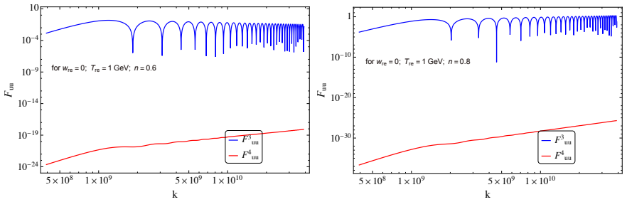
Significance. If the underlying assumptions hold, the paper would be a useful contribution: it connects reheating parameters to the amplitude and tilt of primordial magnetic fields and to a distinctive GW signature. The calculation is not a tautology, since the GW spectrum is obtained through convolution integrals and transfer functions, and the authors provide a numerical check of one key momentum integral (F_uu^1 in Fig. 10). The paper also makes falsifiable spectral predictions, such as a blue-tilted broken power-law GW spectrum peaking near the reheating scale. However, the significance is reduced by three load-bearing caveats: the sawtooth coupling is imposed rather than derived from a field theory, the normalization of B_0 assumes adiabatic evolution for modes that are actually sub-horizon during radiation domination, and a central GW normalization is fixed by a fitted numerical prefactor. These caveats make the claimed viable parameter window and detectability statements provisional.

major comments (3)

[Sec. II.B.a, Eq. (29), Fig. 4] The adiabatic-evolution premise stated in Sec. II.B.a — that these large-scale modes evolve adiabatically because they remain far outside the horizon during the radiation-dominated era — is inconsistent for the scale used in the main constraint, k = 1 Mpc^{-1}. The mode re-entering at matter-radiation equality is k_eq ~ 0.01 Mpc^{-1}, so a 1 Mpc^{-1} mode is already sub-horizon at η ~ 1 Mpc, long before η_eq ~ 100 Mpc. During the radiation-dominated era the universe is a highly conducting plasma, so the field is a sub-horizon magnetic field rather than a super-horizon frozen quantity. The paper's explicit neglect of MHD is therefore not justified for this mode, and turbulent, viscous, resistive, or other non-adiabatic processes can lower B_0 relative to the ρ_B ∝ a^{-4} scaling used in Eq. (29). Because the parameter windows quoted in the Conclusion (wre=0: 0.8<n<0.95, 10^{-2}≤T_re≤10^2 GeV; wre=1/3: 0.5<n<0.55) are selected precisely to keep B_0(1 Mpc^{-1}) above the observational lower bounds while avoiding backreaction, a downward correction to B_0 can eliminate the claimed window, and the GW amplitudes in Eq. (58) and Figs. 7-8, which are normalized using the same parameters, inherit the same fragility.
[Eq. (8), Eqs. (27), (31)] The broken power-law coupling function in Eq. (8) is an external ansatz: the paper provides no Lagrangian, scalar potential, or other microphysical mechanism that produces f(a) ∝ a^n during inflation and f(a) ∝ a^{-m} during reheating, and no derivation of the normalization f(η_re)=1. This normalization is load-bearing because it fixes α = 2nβ/(1+3wre), which controls the enhancement factors (x_re/x_end)^{2(α+1)} in Eq. (27) and the backreaction estimate in Eq. (31). Without a concrete realization, the results are conditional on the existence of such a coupling; the manuscript should state this limitation explicitly or present a model that generates this time dependence. This does not make the calculation internally inconsistent, but it materially weakens the claim that the scenario is a viable mechanism.
[Appendix 2, Eq. (88); Eqs. (58)-(59)] The analytical result for the tensor integral in the k > k_re regime is calibrated with a purely numerical prefactor: the text states that 'we need to include an overall numerical prefactor. We find that this prefactor is approximately 0.2.' This fitted prefactor enters the coefficient A_2 in Eq. (59b) and therefore the amplitude of the secondary GW spectrum for sub-horizon modes in Eq. (58) and Figs. 7-8. The paper does not quantify the uncertainty in this fit, derive it from the Bessel integrals, or show validation over the full parameter range used in the detectability plots. Since the detectability claims involve crossing sensitivity curves by modest margins, a factor-of-a-few error in this prefactor could change the conclusions.

minor comments (5)

[Fig. 7 and Fig. 8 captions] The captions of Fig. 7 and Fig. 8 appear to be identical, while the main text describes different parameter variations in each figure; the captions should be corrected to match the panels.
[Eq. (57) and surrounding text] The text defines a coefficient D, while Eq. (57) uses D_1 for the same or closely related quantity; the notation should be unified.
[Appendix, Eqs. (62)-(88)] The appendix contains several typographical and grammatical errors, such as 'In n Fig. 10' and 'consistence', and some equation references in the text point to the appendix equations with inconsistent numbering; these should be cleaned up.
[Introduction and Eq. (1)] There are minor typographical issues in the introduction, including 'Kinatic coupling' for 'kinetic coupling' and 'FLR W' for 'FLRW'; these should be corrected.
[Eq. (10)] The parameter σ is defined just below Eq. (10), but it would be clearer to define it before first use, since the expression for k_e already depends on it.

Circularity Check

0 steps flagged · score 0.0 of 10

No significant circularity: the magnetic-field and GW spectra are derived from the coupling ansatz and external constraints; GW detectability is a conditional consequence, not an input.

full rationale

The paper's central derivation is self-contained: it solves the gauge-field equation of motion (Eqs. 12-16) with an explicitly stated broken-power-law coupling ansatz (Eq. 8), computes the magnetic and electric spectral energy densities at the end of inflation and reheating (Eqs. 19, 27, 28), and then evaluates the present-day magnetic field via adiabatic scaling (Eq. 29). The secondary gravitational-wave spectra are obtained from the same electromagnetic spectra through the standard anisotropic-stress source integral (Eqs. 37, 47, 50, 58), with the paper explicitly noting that the GW spectral energy density is proportional to the square of the magnetic spectral energy density. The parameter window (n, Tre) is selected to satisfy external observational constraints (CMB anisotropy bound on B0, backreaction, and tensor-to-scalar ratio), not fitted to the GW signal. The GW detectability claim is therefore a conditional consequence of the assumed coupling model and the chosen parameters, not a restatement of the inputs. Self-citations appear for standard reheating and GW-formula expressions (Refs. [26], [85], [91], [92]), but these are technical results that can be independently verified and do not carry the paper's central argument by themselves. No circular step of self-definition, fitted-input-as-prediction, uniqueness-imported-from-authors, or ansatz-smuggling-via-citation was found.

Assumptions & free parameters 5 free parameters · 7 assumptions · 1 invented entities

The central claim rests on the externally prescribed sawtooth coupling, the reheating parametrization, and a set of physical approximations. The only genuinely fitted style parameters are n, Tre, wre, and r0.05, plus the numerical prefactor 0.2 used to match one GW integral. The model does not introduce new particles, but it does posit a new coupling function with no independent evidence.

free parameters (5)

n = 0.8 to 0.95 for wre=0; 0.5 to 0.55 for wre=1/3
Inflationary coupling exponent controlling spectral tilts; chosen to satisfy B0 bounds and backreaction constraints in Table I and Figs. 4-6.
Tre = 10^-2 to 10^2 GeV
Reheating temperature; varied to keep the produced EM energy subdominant and to meet the magnetic field lower bound.
wre = 0 or 1/3
Reheating equation of state; treated as a scenario parameter in the parameter scan.
r0.05 = 0.036 or 10^-4
Tensor-to-scalar ratio used to fix the inflationary Hubble scale HI; varied to show the dependence of B0 and GW amplitudes.
GW numerical prefactor = approximately 0.2
Introduced in Appendix 2 to match the analytic estimate of the F3uu integral to the full numerical result; directly affects GW amplitude.

assumptions (7)

standard math The electromagnetic action has the f(η)^2 F^2 coupling and conformal invariance is broken only by this coupling.
Starting action, Eq. (1), used throughout the derivation.
domain assumption The background is FLRW with de Sitter inflation and power-law reheating, a ∝ η^δ.
Scale-factor evolution used in Eqs. (8), (9), and (21).
standard math Gauge field modes start in the Bunch-Davies vacuum deep inside the horizon.
Initial condition used to fix c1 and c2 in Eq. (15).
ad hoc to paper The sawtooth coupling f(a) is externally imposed, including f(ηre)=1.
Eq. (8) defines the coupling with no Lagrangian or field dynamics; the normalization condition fixes m = nβ.
domain assumption After reheating, the electric field decays due to high conductivity and the magnetic field evolves adiabatically, ρB ∝ a^-4, with MHD effects ignored.
Applied in Section II B a to compute the present-day field strength B0.
domain assumption The electromagnetic anisotropic stress sources GWs only until neutrino decoupling, after which neutrinos balance the anisotropies.
Used in Eq. (47) with integration limit xν = kην, citing refs. [102,103].
domain assumption The reheating epoch is parametrized by wre and Tre through the Dai-Kamionkowski-Wang relations for ke and kre.
Eqs. (10) and (11) are imported from prior literature and set the mode scales.

invented entities (1)

Sawtooth coupling function f(a)
purpose: Breaks conformal invariance during inflation and reheating, generating magnetic fields while keeping f ≥ 1 to avoid strong coupling.
The broken power-law form in Eq. (8) is a postulated ansatz with no microphysical realization; all predictions, B0 and GW spectra, are internal consequences of this assumed function.

how reviews work

0 comments

Cite this review

Pith. "Pith review of Magnetogenesis from Sawtooth Coupling: Gravitational Wave Probe of Reheating." pith.science (2026). https://pith.science/paper/QJOF2MOM

@misc{pith2026250606183,
  author       = {Pith},
  title        = {Pith review of: Magnetogenesis from Sawtooth Coupling: Gravitational Wave Probe of Reheating},
  year         = {2026},
  howpublished = {\url{https://pith.science/paper/QJOF2MOM}},
  note         = {Machine review of arXiv:2506.06183}
}

read the original abstract

The detection of gravitational waves (GWs) by LIGO-Virgo and pulsar timing arrays (PTAs) has opened a new window into early universe cosmology. Yet, the origin of large-scale magnetic fields and the dynamics of the reheating epoch remain poorly understood. In this work, we study the generation of secondary GWs (SGWs) sourced by primordial magnetic fields produced via a Sawtooth-type coupling during reheating with a general background evolution. We show that the reheating equation of state significantly influences the spectral shape and amplitude of the magnetic fields. While a scale-invariant spectrum is typically needed to match observational bounds, this coupling naturally produces a strongly blue-tilted spectrum that remains consistent with current constraints. Crucially, the magnetic field continues to grow during reheating, leading to a GW signal with a broken power-law spectrum and a distinctive blue tilt on super-horizon scales. This SGW signal can fall within the sensitivity of upcoming detectors such as LISA, DECIGO, and BBO. The unique spectral features make this scenario distinguishable from other sources, offering a viable mechanism for cosmic magnetogenesis and a novel probe of the reheating era through GW observations.

Figures

Figures reproduced from arXiv: 2506.06183 by the authors.

**Figure 2.** FIG. 2: Comoving electric and magnetic power spectra, [PITH_FULL_IMAGE:figures/full_fig_p008_2.png] view at source ↗

**Figure 3.** FIG. 3: Comoving electric and magnetic spectral energy density, [PITH_FULL_IMAGE:figures/full_fig_p008_3.png] view at source ↗

Figures from the paper (9 more)

**Figure 4.** Figure 4: FIG. 4: Present-day magnetic field strength [PITH_FULL_IMAGE:figures/full_fig_p010_4.png]

**Figure 5.** Figure 5: FIG. 5: Fractional energy density of the EM field, [PITH_FULL_IMAGE:figures/full_fig_p012_5.png]

**Figure 6.** Figure 6: FIG. 6: Fractional energy density [PITH_FULL_IMAGE:figures/full_fig_p012_6.png]

**Figure 7.** Figure 7: FIG. 7: Gravitational wave spectral energy density Ω [PITH_FULL_IMAGE:figures/full_fig_p018_7.png]

**Figure 8.** Figure 8: FIG. 8: Gravitational wave spectral energy density Ω [PITH_FULL_IMAGE:figures/full_fig_p019_8.png]

**Figure 9.** Figure 9: FIG. 9: In these figures we have plotted [PITH_FULL_IMAGE:figures/full_fig_p021_9.png]

**Figure 10.** Figure 10: FIG. 10: This figure shows how the numerical and analytical results are consistent for a specific set of parameters. [PITH_FULL_IMAGE:figures/full_fig_p022_10.png]

**Figure 11.** Figure 11: FIG. 11: In this figure, we have shown how the numerical and analytical estimate is consistence with each other for a [PITH_FULL_IMAGE:figures/full_fig_p023_11.png]

**Figure 12.** Figure 12: FIG. 12: In this figure, we have shown how the numerical and analytical estimates are consistent for a specific set of [PITH_FULL_IMAGE:figures/full_fig_p024_12.png]

Discussion (0). Sign in to comment.

Forward citations

Cited by 1 Pith paper

Reviewed papers in the Pith corpus that reference this work. Sorted by Pith novelty score. Full citation record

Magnetically assisted primordial scalar perturbations: Scalar-Induced Gravitational Waves
astro-ph.CO 2026-07 conditional novelty 6.0 of 10

PMF-sourced scalar perturbations during a kination-like reheating can induce a gravitational-wave background that dominates over the direct PMF tensor signal and may be detectable at mHz-kHz frequencies.

Reference graph

Works this paper leans on

105 extracted references · 8 canonical work pages · cited by 1 Pith paper

[1]

For such modes, the time integral contributing to the gravitational wave amplitude can be split into two domains: umin ≤ u ≤ 1 and 1 ≤ u ≤ umax

Computing the tensor power spectrum for k < kre: Let us now consider those modes that remain outside the horizon at the end of reheating, i.e., k < kre. For such modes, the time integral contributing to the gravitational wave amplitude can be split into two domains: umin ≤ u ≤ 1 and 1 ≤ u ≤ umax. In this regime, we can safely take the limit xre < 1, as th...
[2]

10: This figure shows how the numerical and analytical results are consistent for a specific set of parameters

× 10-5 k F1uu FIG. 10: This figure shows how the numerical and analytical results are consistent for a specific set of parameters. where we used lim u<1 Z 1 −1 dµf (µ, γ) = Z 1 −1 dµ(1 + µ2)(1 + γ2) ≃ Z 1 −1 dµ(1 + µ2) ≃ 8 3 (68) lim u<1 Z 1 −1 dµf (µ, γ) = Z 1 −1 dµ(1 + µ2)(1 + γ2) ≃ Z 1 −1 dµ(1 + µ2)2 ≃ 16 15 (69) γ = \k − q · ˆk = k − q |k − q| · ˆk = ...
[3]

Computing the tensor power spectrum for k > kre: We now turn our attention to scenarios where all relevant modes are deep inside the horizon before the end of reheating, i.e., k > kre, which corresponds to xre > 1. In this regime, the tensor power spectrum sourced by 22 F3uu F4uu forw re =0;T re =1 GeV;n=0.6 5 × 108 1 × 109 5 × 109 1 × 1010 10-24 10-19 10...
[4]

Giovannini, Int

M. Giovannini, Int. J. Mod. Phys. D 13, 391 (2004), arXiv:astro-ph/0312614 . 24

arXiv 2004
[5]

Grasso and H

D. Grasso and H. R. Rubinstein, Phys. Rept. 348, 163 (2001), arXiv:astro-ph/0009061

arXiv 2001
[6]

P. P. Kronberg, Q. W. Dufton, H. Li, and S. A. Colgate, Astrophys. J. 560, 178 (2001), arXiv:astro-ph/0106281

work page Pith review arXiv 2001
[7]

Durrer and A

R. Durrer and A. Neronov, Astron. Astrophys. Rev. 21, 62 (2013), arXiv:1303.7121 [astro-ph.CO]

arXiv 2013
[8]

Subramanian, Rept

K. Subramanian, Rept. Prog. Phys. 79, 076901 (2016), arXiv:1504.02311 [astro-ph.CO]

arXiv 2016

Show all 105 references

[10]

Neronov and I

A. Neronov and I. Vovk, Science 328, 73 (2010), arXiv:1006.3504 [astro-ph.HE]

2010 arXiv
[11]

Tavecchio, G

F. Tavecchio, G. Ghisellini, L. Foschini, G. Bonnoli, G. Ghirlanda, and P. Coppi, Mon. Not. Roy. Astron. Soc. 406, L70 (2010), arXiv:1004.1329 [astro-ph.CO]

2010 arXiv
[12]

Dolag, M

K. Dolag, M. Kachelriess, S. Ostapchenko, and R. Tomas, Astrophys. J. Lett. 727, L4 (2011), arXiv:1009.1782 [astro-ph.HE]

2011 arXiv
[13]

C. D. Dermer, M. Cavadini, S. Razzaque, J. D. Finke, J. Chiang, and B. Lott, Astrophys. J. Lett. 733, L21 (2011), arXiv:1011.6660 [astro-ph.HE]

2011 arXiv
[14]

I. Vovk, A. M. Taylor, D. Semikoz, and A. Neronov, Astrophys. J. Lett. 747, L14 (2012), arXiv:1112.2534 [astro- ph.CO]

2012 arXiv
[15]

A. M. Taylor, I. Vovk, and A. Neronov, Astron. Astrophys. 529, A144 (2011), arXiv:1101.0932 [astro-ph.HE]

2011 arXiv
[16]

Takahashi, M

K. Takahashi, M. Mori, K. Ichiki, and S. Inoue, Astrophys. J. Lett. 744, L7 (2012), arXiv:1103.3835 [astro-ph.CO]

2012 arXiv
[17]

Paoletti, J

D. Paoletti, J. Chluba, F. Finelli, and J. Rubi˜ no-Mart ´ ın, Monthly Notices of the Royal Astronomical Society517, 3916 (2022)

2022
[18]

Zucca, Y

A. Zucca, Y. Li, and L. Pogosian, Phys. Rev. D 95, 063506 (2017), arXiv:1611.00757 [astro-ph.CO]

2017 arXiv
[19]

M. S. Turner and L. M. Widrow, Phys. Rev. D 37, 2743 (1988)

1988
[20]

Papanikolaou, C

T. Papanikolaou, C. Tzerefos, S. Capozziello, and G. Lambiase, JCAP 01, 051 (2025), arXiv:2408.17259 [astro- ph.CO]

2025 arXiv
[21]

Demozzi, V

V. Demozzi, V. Mukhanov, and H. Rubinstein, JCAP 08, 025 (2009), arXiv:0907.1030 [astro-ph.CO]

2009 arXiv
[22]

Ratra, Astrophys

B. Ratra, Astrophys. J. Lett. 391, L1 (1992)

1992
[23]

Kandus, K

A. Kandus, K. E. Kunze, and C. G. Tsagas, Phys. Rept. 505, 1 (2011), arXiv:1007.3891 [astro-ph.CO]

2011 arXiv
[24]

R. J. Z. Ferreira, R. K. Jain, and M. S. Sloth, JCAP 10, 004 (2013), arXiv:1305.7151 [astro-ph.CO]

2013 arXiv
[25]

Kobayashi, JCAP 05, 040 (2014), arXiv:1403.5168 [astro-ph.CO]

T. Kobayashi, JCAP 05, 040 (2014), arXiv:1403.5168 [astro-ph.CO]

2014 arXiv
[26]

M. R. Haque, D. Maity, and S. Pal, Phys. Rev. D 103, 103540 (2021), arXiv:2012.10859 [hep-th]

2021 arXiv
[27]

Tripathy, D

S. Tripathy, D. Chowdhury, R. K. Jain, and L. Sriramkumar, Phys. Rev. D 105, 063519 (2022), arXiv:2111.01478 [astro-ph.CO]

2022 arXiv
[28]

Li and L.-Y

Y. Li and L.-Y. Zhang, Mod. Phys. Lett. A 37, 2250069 (2022)

2022
[29]

Maiti, D

S. Maiti, D. Maity, and R. Srikanth, (2025), arXiv:2505.13623 [astro-ph.CO]

2025
[30]

Sharma, S

R. Sharma, S. Jagannathan, T. R. Seshadri, and K. Subramanian, Phys. Rev. D 96, 083511 (2017), arXiv:1708.08119 [astro-ph.CO]

2017 arXiv
[31]

Dimopoulos, A

K. Dimopoulos, A. Ghoshal, and T. Papanikolaou, Phys. Rev. D 111, 083550 (2025)

2025
[32]

Cecchini and M

C. Cecchini and M. Rinaldi, Phys. Dark Univ. 40, 101212 (2023), arXiv:2301.07699 [astro-ph.CO]

2023 arXiv
[33]

Campanelli, Int

L. Campanelli, Int. J. Mod. Phys. D 18, 1395 (2009), arXiv:0805.0575 [astro-ph]

2009 arXiv
[34]

R. K. Jain, R. Durrer, and L. Hollenstein, J. Phys. Conf. Ser. 484, 012062 (2014), arXiv:1204.2409 [astro-ph.CO]

2014 arXiv
[35]

Caprini and L

C. Caprini and L. Sorbo, JCAP 10, 056 (2014), arXiv:1407.2809 [astro-ph.CO]

2014 arXiv
[36]

Sharma, K

R. Sharma, K. Subramanian, and T. R. Seshadri, Phys. Rev. D 97, 083503 (2018), arXiv:1802.04847 [astro-ph.CO]

2018 arXiv
[37]

Bamba, S

K. Bamba, S. D. Odintsov, T. Paul, and D. Maity, Phys. Dark Univ. 36, 101025 (2022), arXiv:2107.11524 [gr-qc]

2022 arXiv
[38]

Adshead, J

P. Adshead, J. T. Giblin, T. R. Scully, and E. I. Sfakianakis, JCAP 10, 039 (2016), arXiv:1606.08474 [astro-ph.CO]

2016 arXiv
[39]

G. Baym, D. B¨ odeker, and L. McLerran, Phys. Rev. D 53, 662 (1996)

1996
[40]

Ahonen and K

J. Ahonen and K. Enqvist, Phys. Rev. D 57, 664 (1998), arXiv:hep-ph/9704334 [hep-ph]

1998 arXiv
[41]

Yang and L

J. Yang and L. Bian, Phys. Rev. D 106, 023510 (2022), arXiv:2102.01398 [astro-ph.CO]

2022 arXiv
[42]

J. M. Quashnock, A. Loeb, and D. N. Spergel, Astrophys. J. Lett. 344, L49 (1989)

1989
[43]

Fu, Y.-x

W.-j. Fu, Y.-x. Liu, and Y.-l. Wu, Int. J. Mod. Phys. A 26, 4335 (2011), arXiv:1003.4169 [hep-ph]

2011 arXiv
[44]

A. K. Pandey and S. Anand, Phys. Rev. D 104, 063508 (2021)

2021
[45]

Christensson, M

M. Christensson, M. Hindmarsh, and A. Brandenburg, Phys. Rev. E 64, 056405 (2001)

2001
[46]

Caprini, R

C. Caprini, R. Durrer, and G. Servant, JCAP 12, 024 (2009), arXiv:0909.0622 [astro-ph.CO]

2009 arXiv
[47]

Brandenburg, K

A. Brandenburg, K. Enqvist, and P. Olesen, Phys. Rev. D 54, 1291 (1996), arXiv:astro-ph/9602031

1996 arXiv
[48]

Caprini and R

C. Caprini and R. Durrer, Phys. Rev. D 65, 023517 (2001), arXiv:astro-ph/0106244

2001 arXiv
[49]

A. H. Guth, Phys. Rev. D 23, 347 (1981)

1981
[50]

A. D. Linde, Phys. Lett. B 108, 389 (1982)

1982
[51]

Albrecht and P

A. Albrecht and P. J. Steinhardt, Phys. Rev. Lett. 48, 1220 (1982)

1982
[52]

A. A. Starobinsky, Phys. Lett. B 91, 99 (1980)

1980
[53]

A. R. Liddle, P. Parsons, and J. D. Barrow, Phys. Rev. D 50, 7222 (1994)

1994
[54]

Kobayashi and M

T. Kobayashi and M. S. Sloth, Phys. Rev. D 100, 023524 (2019). 25

2019
[55]

Maity, S

D. Maity, S. Pal, and T. Paul, JCAP 05, 045 (2021), arXiv:2103.02411 [hep-th]

2021 arXiv
[56]

Benevides, A

A. Benevides, A. Dabholkar, and T. Kobayashi, JHEP 11, 039 (2018), arXiv:1808.08237 [hep-th]

2018 arXiv
[57]

Kobayashi and M

T. Kobayashi and M. S. Sloth, Phys. Rev. D 100, 023524 (2019), arXiv:1903.02561 [astro-ph.CO]

2019 arXiv
[58]

Fujita and R

T. Fujita and R. Namba, Phys. Rev. D 94, 043523 (2016)

2016
[59]

H. J. Hort´ ua and L. Casta˜ neda, Phys. Rev. D90, 123520 (2014), arXiv:1405.1786 [gr-qc]

2014 arXiv
[60]

L. Dai, M. Kamionkowski, and J. Wang, Phys. Rev. Lett. 113, 041302 (2014)

2014
[61]

Martin and C

J. Martin and C. Ringeval, Phys. Rev. D 82, 023511 (2010)

2010
[62]

Maity and P

D. Maity and P. Saha, Phys. Rev. D 98, 103525 (2018)

2018
[63]

M. R. Haque and D. Maity, Phys. Rev. D 107, 043531 (2023)

2023
[64]

Lentati et al., Mon

L. Lentati et al., Mon. Not. Roy. Astron. Soc. 453, 2576 (2015), arXiv:1504.03692 [astro-ph.CO]

2015 arXiv
[65]

Arzoumanian et al

Z. Arzoumanian et al. (NANOGrav), Astrophys. J. Lett. 905, L34 (2020), arXiv:2009.04496 [astro-ph.HE]

2020 arXiv
[66]

Agazie et al

G. Agazie et al. (NANOGrav), Astrophys. J. Lett. 951, L8 (2023), arXiv:2306.16213 [astro-ph.HE]

2023 arXiv
[67]

et al, arXiv e-prints , arXiv:2306.16224 (2023), arXiv:2306.16224 [astro-ph.HE]

A. et al, arXiv e-prints , arXiv:2306.16224 (2023), arXiv:2306.16224 [astro-ph.HE]

2023 arXiv
[68]

D. J. Reardon et al., Astrophys. J. Lett. 951, L6 (2023), arXiv:2306.16215 [astro-ph.HE]

2023 arXiv
[69]

Zic et al., (2023), arXiv:2306.16230 [astro-ph.HE]

A. Zic et al., (2023), arXiv:2306.16230 [astro-ph.HE]

2023 arXiv
[70]

Xu et al., Res

H. Xu et al., Res. Astron. Astrophys. 23, 075024 (2023), arXiv:2306.16216 [astro-ph.HE]

2023 arXiv
[71]

Janssen et al., PoS AASKA14, 037 (2015), arXiv:1501.00127 [astro-ph.IM]

G. Janssen et al., PoS AASKA14, 037 (2015), arXiv:1501.00127 [astro-ph.IM]

2015 arXiv
[72]

Amaro-Seoane et al., GW Notes 6, 4 (2013), arXiv:1201.3621 [astro-ph.CO]

P. Amaro-Seoane et al., GW Notes 6, 4 (2013), arXiv:1201.3621 [astro-ph.CO]

2013 arXiv
[73]

Barausse et al., Gen

E. Barausse et al., Gen. Rel. Grav. 52, 81 (2020), arXiv:2001.09793 [gr-qc]

2020 arXiv
[74]

Crowder and N

J. Crowder and N. J. Cornish, Phys. Rev. D 72, 083005 (2005), arXiv:gr-qc/0506015

2005 arXiv
[75]

Corbin and N

V. Corbin and N. J. Cornish, Class. Quant. Grav. 23, 2435 (2006), arXiv:gr-qc/0512039

2006 arXiv
[76]

Baker et al., Bull

J. Baker et al., Bull. Am. Astron. Soc. 51, 243 (2019), arXiv:1907.11305 [astro-ph.IM]

2019 arXiv
[77]

N. Seto, S. Kawamura, and T. Nakamura, Phys. Rev. Lett. 87, 221103 (2001), arXiv:astro-ph/0108011

2001 arXiv
[78]

Kawamura et al., Class

S. Kawamura et al., Class. Quant. Grav. 28, 094011 (2011)

2011
[79]

Suemasa, K

A. Suemasa, K. Nakagawa, and M. Musha, Proc. SPIE Int. Soc. Opt. Eng. 10563, 105632V (2017)

2017
[80]

Punturo et al., Class

M. Punturo et al., Class. Quant. Grav. 27, 194002 (2010)

2010
[81]

Sathyaprakash et al., Class

B. Sathyaprakash et al., Class. Quant. Grav. 29, 124013 (2012), [Erratum: Class.Quant.Grav. 30, 079501 (2013)], arXiv:1206.0331 [gr-qc]

2012 arXiv
[82]

Blas and A

D. Blas and A. C. Jenkins, Phys. Rev. Lett. 128, 101103 (2022), arXiv:2107.04601 [astro-ph.CO]

2022 arXiv
[83]

J. W. Foster, D. Blas, A. Bourgoin, A. Hees, M. Herrero-Valea, A. C. Jenkins, and X. Xue, (2025), arXiv:2504.15334 [astro-ph.CO]

2025 arXiv
[84]

K. Choi, H. Kim, and T. Sekiguchi, Phys. Rev. Lett. 121, 031102 (2018)

2018
[85]

Patel, H

T. Patel, H. Tashiro, and Y. Urakawa, JCAP 01, 043 (2020), arXiv:1909.00288 [astro-ph.CO]

2020 arXiv
[86]

Brandenburg, O

A. Brandenburg, O. Iarygina, E. I. Sfakianakis, and R. Sharma, JCAP 12, 057 (2024), arXiv:2408.17413 [astro- ph.CO]

2024 arXiv
[87]

P. A. R. Ade et al. (BICEP2, Keck Arrary), Phys. Rev. D 96, 102003 (2017), arXiv:1705.02523 [astro-ph.CO]

2017 arXiv
[88]

Chakraborty, S

A. Chakraborty, S. Maiti, and D. Maity, Phys. Rev. D 111, 083505 (2025), arXiv:2408.07767 [astro-ph.CO]

2025 arXiv
[89]

Martin and J

J. Martin and J. Yokoyama, JCAP 01, 025 (2008), arXiv:0711.4307 [astro-ph]

2008 arXiv
[90]

Sorbo, JCAP 06, 003 (2011), arXiv:1101.1525 [astro-ph.CO]

L. Sorbo, JCAP 06, 003 (2011), arXiv:1101.1525 [astro-ph.CO]

2011 arXiv
[91]

Ito and J

A. Ito and J. Soda, Phys. Lett. B 771, 415 (2017), arXiv:1607.07062 [hep-th]

2017 arXiv
[92]

Sharma, K

R. Sharma, K. Subramanian, and T. R. Seshadri, Phys. Rev. D 101, 103526 (2020), arXiv:1912.12089 [astro-ph.CO]

2020 arXiv
[93]

Okano and T

S. Okano and T. Fujita, JCAP 03, 026 (2021), arXiv:2005.13833 [astro-ph.CO]

2021 arXiv
[94]

Maiti, D

S. Maiti, D. Maity, and R. Srikanth, (2025), arXiv:2504.15400 [astro-ph.CO]

2025 arXiv
[95]

Maiti, D

S. Maiti, D. Maity, and L. Sriramkumar, (2024), arXiv:2401.01864 [gr-qc]

2024 arXiv
[96]

A. A. Starobinsky, JETP Lett. 30, 682 (1979)

1979
[97]

L. P. Grishchuk, Zh. Eksp. Teor. Fiz. 67, 825 (1974)

1974
[98]

M. C. Guzzetti, N. Bartolo, M. Liguori, and S. Matarrese, Riv. Nuovo Cim. 39, 399 (2016), arXiv:1605.01615 [astro-ph.CO]

2016 arXiv
[99]

M. R. Haque, D. Maity, T. Paul, and L. Sriramkumar, Phys. Rev. D 104, 063513 (2021), arXiv:2105.09242 [astro-ph.CO]

2021 arXiv
[100]

A. A. Starobinskii, ZhETF Pisma Redaktsiiu 30, 719 (1979)

1979
[101]

P. A. R. Ade et al. (Planck), Astron. Astrophys. 594, A13 (2016), arXiv:1502.01589 [astro-ph.CO]

2016 arXiv
[102]

P. A. R. Ade et al. (BICEP, Keck), Phys. Rev. Lett. 127, 151301 (2021), arXiv:2110.00483 [astro-ph.CO]

2021
[103]

P. A. R. Ade et al.(BICEP2, Keck Array), Phys. Rev. Lett. 121, 221301 (2018), arXiv:1810.05216 [astro-ph.CO]

2018 arXiv
[104]

Akrami et al

Y. Akrami et al. (Planck), Astron. Astrophys. 641, A10 (2020), arXiv:1807.06211 [astro-ph.CO]

2020 arXiv
[105]

Lewis, Phys

A. Lewis, Phys. Rev. D 70, 043011 (2004)

2004
[106]

Abbott et al

R. Abbott et al. (KAGRA, Virgo, LIGO Scientific), Phys. Rev. D 104, 022004 (2021), arXiv:2101.12130 [gr-qc] . 26

2021

Pith tools

Reviewed August 7, 2026 · model on record in the stance chip above.

[1] [1]

For such modes, the time integral contributing to the gravitational wave amplitude can be split into two domains: umin ≤ u ≤ 1 and 1 ≤ u ≤ umax

Computing the tensor power spectrum for k < kre: Let us now consider those modes that remain outside the horizon at the end of reheating, i.e., k < kre. For such modes, the time integral contributing to the gravitational wave amplitude can be split into two domains: umin ≤ u ≤ 1 and 1 ≤ u ≤ umax. In this regime, we can safely take the limit xre < 1, as th...

[2] [2]

10: This figure shows how the numerical and analytical results are consistent for a specific set of parameters

× 10-5 k F1uu FIG. 10: This figure shows how the numerical and analytical results are consistent for a specific set of parameters. where we used lim u<1 Z 1 −1 dµf (µ, γ) = Z 1 −1 dµ(1 + µ2)(1 + γ2) ≃ Z 1 −1 dµ(1 + µ2) ≃ 8 3 (68) lim u<1 Z 1 −1 dµf (µ, γ) = Z 1 −1 dµ(1 + µ2)(1 + γ2) ≃ Z 1 −1 dµ(1 + µ2)2 ≃ 16 15 (69) γ = \k − q · ˆk = k − q |k − q| · ˆk = ...

[3] [3]

Computing the tensor power spectrum for k > kre: We now turn our attention to scenarios where all relevant modes are deep inside the horizon before the end of reheating, i.e., k > kre, which corresponds to xre > 1. In this regime, the tensor power spectrum sourced by 22 F3uu F4uu forw re =0;T re =1 GeV;n=0.6 5 × 108 1 × 109 5 × 109 1 × 1010 10-24 10-19 10...

[4] [4]

Giovannini, Int

M. Giovannini, Int. J. Mod. Phys. D 13, 391 (2004), arXiv:astro-ph/0312614 . 24

arXiv 2004

[5] [5]

Grasso and H

D. Grasso and H. R. Rubinstein, Phys. Rept. 348, 163 (2001), arXiv:astro-ph/0009061

arXiv 2001

[6] [6]

P. P. Kronberg, Q. W. Dufton, H. Li, and S. A. Colgate, Astrophys. J. 560, 178 (2001), arXiv:astro-ph/0106281

work page Pith review arXiv 2001

[7] [7]

Durrer and A

R. Durrer and A. Neronov, Astron. Astrophys. Rev. 21, 62 (2013), arXiv:1303.7121 [astro-ph.CO]

arXiv 2013

[8] [8]

Subramanian, Rept

K. Subramanian, Rept. Prog. Phys. 79, 076901 (2016), arXiv:1504.02311 [astro-ph.CO]

arXiv 2016