REVIEW 4 major objections 6 minor 29 references
Physics-Informed Neural Networks for Control of Single-Phase Flow Systems Governed by Partial Differential Equations
T0 review · 4 major / 6 minor · reviewed 2026-08-07 · deepseek-v4-flash
Pith's one-line read The paper claims that a two-stage physics-informed neural network, trained only on conservation laws with no labeled data, can replace iterative PDE solvers inside a real-time model predictive controller for single-phase pipe flow.
desk verdict The core PINC-to-PDE extension is real and the accuracy numbers are credible, but the unquantified steady-state-initialization assumption and a feedback loop that Eq. (37) does not actually implement mean the paper needs major revision. read the letter →
The pith
A machine-rendered reading of the paper's core claim, the machinery that carries it, and where it could break.
The reading
What carries the argument
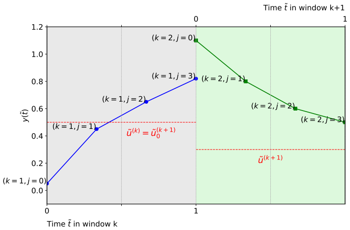
The mechanism is the two-stage PINC architecture with the steady-state-to-transient initialization shortcut. The steady-state network $f(\tilde{x},\tilde{u})$ learns equilibrium pressure and velocity profiles across downstream pressure controls, while the transient network $f(\tilde{x},\tilde{t},\tilde{u}_0,\tilde{u})$ learns the evolution within a normalized time window, where $\tilde{u}_0$ is the previous window's control and $\tilde{u}$ is the current control. The initial-condition loss of the transient network is computed by evaluating the frozen steady-state network at $(\tilde{x},\tilde{u}_0)$, so the spatial initial profile is never an input. This is what cuts the input dimensionality from a discretized spatial field to a single scalar and what breaks autoregressive feedback, making long-term simulation a sequence of independent window evaluations.
What would settle it
Run the finite-difference plant with a control sequence whose window duration is shorter than the system's settling time, starting from a state far from the steady profile implied by the previous control; if the open-loop PINC window predictions then drift well beyond the reported 93% fit compare, the steady-state-initialization assumption is the cause. In the incompressible 1 second sampling case, comparing the PINC prediction against the plant at a non-equilibrium initial condition directly tests whether the four-input surrogate still holds.
Extended reading notes
Core claim
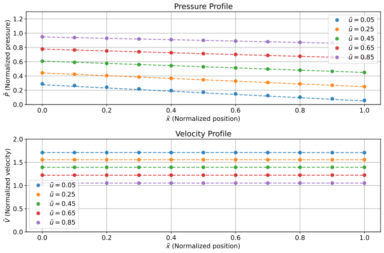
The central discovery, stated in the authors' terms, is that PINC for PDEs can be trained without labeled data to represent transient single-phase flow and can be used directly for model predictive control. Steady-state mean absolute percentage error is below 1.1% for both incompressible and compressible cases, transient fit compare exceeds 93% against a finite-difference plant, and the surrogate is 7 to 188 times faster at inference. Because the transient network's outputs depend only on previous and current control inputs, not on fed-back predictions, the authors argue there is no error accumulation during forward simulation; each control window restarts from the steady state implied by the previous control. This permits arbitrarily long horizon simulations by cascading windows, and closed-loop MPC experiments show the controller can steer a measured downhole pressure toward an unattainable low target while respecting rate-of-change constraints.
Load-bearing premise
The load-bearing premise is that at the start of every control window the system sits exactly at the steady state reached under the previous constant control, so the previous control value alone fully describes the initial condition.
Editorial extensions
If this is right
- If the claim holds, PDE-constrained flow control no longer needs an iterative numerical solver inside the optimization loop; the MPC can query the network directly and obtain derivatives by automatic differentiation.
- Long-horizon simulations of these flow systems become non-autoregressive, so errors made in one control window do not contaminate the next window.
- The two-stage trick extends the method's scope: any PDE system whose dynamics are driven by boundary controls and whose transient windows start from equilibrium can be cast in the same four-input form.
- The reported speedups, ranging from 7.6 for incompressible steady state to 188 for compressible transient, make the surrogate a candidate for real-time monitoring and optimization rather than only offline simulation.
Reading between the lines
- Beyond the paper, a natural test is to replace the steady-state initialization with a true spatial initial profile for a few windows and measure how much accuracy is lost, which would quantify the cost of the simplifying assumption.
- The steady-state assumption suggests the framework is best suited to slow control updates; the paper itself notes larger deviations at 1 second sampling in the incompressible case, and a tighter analysis could map exactly where the approximation breaks.
- The same architecture should transfer to other boundary-controlled PDEs, such as heat or wave equations with inlet controls, reusing the steady-state-to-transient bootstrap; the paper hints at this generality but does not demonstrate it.
- Because the network is trained only against PDE residuals and compared against a numeric plant, the accuracy ceiling is set by how well the finite-difference plant itself resolves the equations; validation against real field measurements remains an open step.
Editorial analysis
A structured set of objections, weighed in public.
Referee Report
Summary. The paper extends the Physics-Informed Neural Nets for Control (PINC) framework from ODEs to PDEs, targeting single-phase incompressible and compressible flow in pipelines. The proposed method trains two networks: a steady-state PINC that maps spatial position and outlet pressure (the control variable) to equilibrium pressure and velocity, and a transient PINC that maps position, time, the previous control u0, and the current control u to the state trajectory. The initial condition for each control window is set to the steady-state solution under u0 (Eq. 34, Section 4.4.2), which drastically reduces input dimensionality. The transient PINC is then used inside a model predictive controller. Validation against finite-difference simulations reports steady-state MAPE below 1.1% (Table 4), transient Fit Compare above 93% (Table 5), and inference speedups of 7–188x. The paper emphasizes that the forward simulation has 'no error accumulation' because outputs depend only on u0 and u, not on autoregressive feedback.
Significance. The paper addresses a relevant problem — constructing fast, differentiable surrogate models for PDE-governed systems that can be used for real-time MPC. Its strengths are the physics-only training (no labeled data), the two-stage training scheme that avoids high-dimensional initial-condition inputs, and the external validation against finite-difference solutions, which is a credible benchmark. The reported speedups and accuracy values are promising. However, the central simplifying assumption — that each control window starts from the steady state under the previous control — is structural, and several claims about error accumulation and MPC feedback are currently overstated. These issues are load-bearing and need to be resolved or carefully scoped before the results can be accepted as stated.
major comments (4)
- [Section 4.4.2, Eq. (34)] The steady-state initialization assumption is structural and unquantified. The paper states in Section 4.4.2 that the assumption is valid only if the time window length T is sufficiently large for the system to reach stability, but no settling-time analysis is provided. In the MPC experiments, the sampling time is Ts=1s for the incompressible case and Ts=10s for the compressible case, which correspond to normalized window durations of 0.1 (since tref=10s and 100s, respectively), while the open-loop validation in Figure 10 uses a 10s window (normalized duration 1.0). The paper itself notes in Section 5.1.2 that larger deviations occur at 1s sampling. Because the transient PINC has no mechanism to represent off-steady-state initial conditions, the accuracy reported for the 10s window does not automatically transfer to the sampling time actually used in MPC. Please quantify the settling time for the two test cases and provide a systematic study of prediction accuracy as a function of window length.
- [Algorithm 2, Eq. (37)] The MPC feedback is not actually fed into the predictive model. In Algorithm 2, step 4 sets y0 to the measured output, but in Eq. (37) y0 appears only in the first-step rate constraints |f(xbar,Ts,u0,u1)-y0| <= Δy_max; the predictive model f(x,t,u0,u) does not take the measured state as an input. Therefore the statement in Section 5.1.2 that 'as feedback from the plant is incorporated at each sampling time, these deviations are dynamically corrected' is not supported by the algorithm as written. Either implement a genuine state-correction mechanism (e.g., an additive bias correction of the PINC output using the measured y0) or explicitly limit the claim to say that feedback is used only for the rate constraints, not for correcting the model's state trajectory.
- [Section 4.4.3, Algorithm 1] The 'no error accumulation during PINC inference' contribution is a direct consequence of discarding the state between windows, rather than an accuracy improvement. Because each window's initial condition is reset to the steady state under u0, the PINC forward simulation is not a continuous integration of the actual plant state; it is a sequence of independent steady-state-to-transient segments. Errors do not propagate from window to window only because the state is not carried forward. The claim should be restated as 'the model has no autoregressive state dependency' and the forward simulation should be validated for the same control sequence and sampling time used in the MPC, not only for the 10s-window case shown in Figure 10.
- [Section 5.1.2 and Table 5] The transient accuracy metrics (Fit Compare >93%) are computed for a 10s window (tref=10s), but the MPC controller uses Ts=1s. No quantitative comparison of the PINC vs. the finite-difference plant at Ts=1s is given, and no closed-loop metrics such as tracking error, constraint violations, or comparison against a conventional MPC baseline are reported. Since the central claim of real-time MPC rests on the model's accuracy at the actual sampling time, please provide a quantitative evaluation of PINC predictions at Ts=1s (and Ts=10s for the compressible case) and report closed-loop performance metrics.
minor comments (6)
- [Section 2.2, Eqs. (9) and (16)] The IPR boundary condition is first defined in terms of mass flow rate (Eq. 9) and later in velocity form for the incompressible case (Eq. 16); the relationship between the proportionality constants k and PI should be stated explicitly to avoid confusion.
- [Section 5.1.1] The Reynolds number clamping bounds used in torch.clamp are not specified, even though they are a free hyperparameter that directly affects the friction factor and thus the training dynamics; please report the chosen bounds.
- [Section 5.2.1, Eqs. (39)-(43)] The sinusoidal activation function is defined as f(x)=w1*sin(x)+w2*cos(x), but the equations for the skip-connection architecture use a generic phi; clarify how the sinusoidal activation is incorporated into the forward pass.
- [Figure 13] The red dashed line at x=1 appears to be the control input (outlet pressure) rather than a PINC prediction; the caption should state this explicitly to avoid misreading.
- [Section 4.4.2] The statement that 'many transient simulation applications in practice consider the steady-state regime as the initial condition' would benefit from concrete references or examples beyond the single cited wellbore/reservoir paper.
- [Section 5.3, Table 5] The Fit Compare values are reported as averages over spatial positions, but the spread (e.g., minimum and maximum across positions) is not given; adding this information would help assess spatial consistency.
Circularity Check
Partial self-reference: transient IC targets come from the authors' own steady-state PINC, and the 'no error accumulation' advantage is architectural, but central accuracy/MPC claims are validated against an independent finite-difference plant.
-
self definitional
[Section 4.4, Eq. (34), and Section 4.4.2]
"The initial condition y(˜x,0,˜u0,˜u) must match the steady-state solution obtained from the previously trained steady-state PINC model ... where ȳSS_i(˜xm,˜u^m_0) represents the steady-state solution obtained from the previously trained (with fixed weights) steady-state PINC model."
The transient network's t=0 target is not an independent solution of the PDE but the output of another network trained in the same framework. By construction, the transient PINC is trained so that y(x,0,u0,u) approximates the steady-state PINC output; therefore any evaluation that compares the transient at t=0 with the steady-state PINC is checking a training objective, not a prediction. This is partial circularity: the paper's headline transient accuracy is also measured against a finite-difference plant, so the loop is not closed.
-
self definitional
[Section 4.4.3 (Forward Simulation), Algorithm 1; contribution bullet in Section 1]
"there is no auto-regressive feedback in the model, meaning that the output at the beginning of a new time window, y^(k+1,0), is not the same as the final output of the previous window, y^(k,M−1). This implies that any errors made during one time window do not accumulate or propagate to the next as time progresses. Instead, the initial condition for time window k relies solely on the control value u^(k)_0."
Equation (36) defines y^(k,j)=f(x˜,t˜_j,u0^(k),u^(k)) and Algorithm 1 sets u0^(k+1)=u^(k). The previous window's output y^(k,M-1) is never an input to the next window, so the absence of error accumulation is the direct statement of the non-feedback architecture, not an empirical finding. The paper presents this definitional property as a contribution; it is true by construction and independent of model accuracy.
full rationale
The central modeling and MPC claims are not circular: the PINC models are trained on PDE residuals and boundary/initial-condition losses, and the reported MAPE/Fit Compare values are computed against a finite-difference numerical plant, an external reference not used to fit the networks. The steady-state PINC is itself validated against that plant, so using it to generate IC targets is a transfer of an independently checked surrogate rather than a closed self-justification. Nevertheless, two self-referential elements are present. First, Eq. (34) anchors the transient initial condition to the authors' own steady-state network; the t=0 behavior of the transient model is therefore a training objective with respect to that network, even though later-time dynamics are still constrained by the PDE. Second, the advertised no-error-accumulation property is entailed by the absence of autoregressive feedback in Algorithm 1, so it is an architectural tautology rather than a measured result. The paper also states that the steady-state-initialization assumption requires a sufficiently large window and acknowledges larger deviations at 1 s sampling; this is a correctness/validity limitation, not an additional circularity. No load-bearing self-citation chain or imported uniqueness theorem was found; Antonelo et al. (2024) is background for the PINC concept, not the evidence for the present results. Overall, the derivation has partial self-reference but retains independent empirical content, giving a score of 3.
Assumptions & free parameters
free parameters (4)
- Loss weights lambda_F, lambda_B, lambda_I for transient PINC =
not reported
- Time window length T (normalized tref) =
10 s incompressible, 100 s compressible
- Reynolds number clamp bounds in torch.clamp =
not specified
- Optuna-selected hyperparameters =
layers 8, hidden 43/93, activation tanh/swish, skip true/false, etc.
assumptions (4)
- ad hoc to paper Initial condition for each control window equals the steady-state solution of the previous control u0 (Eq. 34, Section 4.4.2).
- domain assumption Isothermal flow with ideal gas EOS for gas and constant density for liquid.
- domain assumption The friction factor is given by the Blasius or Swamee-Jain correlation and depends on the network outputs.
- domain assumption IPR boundary condition at the inlet and specified outlet pressure as control.
Cite this review
Pith. "Pith review of Physics-Informed Neural Networks for Control of Single-Phase Flow Systems Governed by Partial Differential Equations." pith.science (2026). https://pith.science/paper/ZCKMQMJW
@misc{pith2026250606188,
  author       = {Pith},
  title        = {Pith review of: Physics-Informed Neural Networks for Control of Single-Phase Flow Systems Governed by Partial Differential Equations},
  year         = {2026},
  howpublished = {\url{https://pith.science/paper/ZCKMQMJW}},
  note         = {Machine review of arXiv:2506.06188}
}
read the original abstract
The modeling and control of single-phase flow systems governed by Partial Differential Equations (PDEs) present challenges, especially under transient conditions. In this work, we extend the Physics-Informed Neural Nets for Control (PINC) framework, originally proposed to modeling and control of Ordinary Differential Equations (ODE) without the need of any labeled data, to the PDE case, particularly to single-phase incompressible and compressible flows, integrating neural networks with physical conservation laws. The PINC model for PDEs is structured into two stages: a steady-state network, which learns equilibrium solutions for a wide range of control inputs, and a transient network, which captures dynamic responses under time-varying boundary conditions. We propose a simplifying assumption that reduces the dimensionality of the spatial coordinate regarding the initial condition, allowing the efficient training of the PINC network. This simplification enables the derivation of optimal control policies using Model Predictive Control (MPC). We validate our approach through numerical experiments, demonstrating that the PINC model, which is trained exclusively using physical laws, i.e., without labeled data, accurately represents flow dynamics and enables real-time control applications. The results highlight the PINC's capability to efficiently approximate PDE solutions without requiring iterative solvers, making it a promising alternative for fluid flow monitoring and optimization in engineering applications.
Figures


Figures from the paper (11 more)




Reference graph
Works this paper leans on
-
[6]
Engineering Ap- plications of Artificial Intelligence 138, 109378
Learn- ing characteristic parameters and dynamics of centrifugal pumps under multiphase flow using physics-informed neural networks. Engineering Ap- plications of Artificial Intelligence 138, 109378. doi:10.1016/j.engappai. 2024.109378. Colebrook, C.F., White, C.M.,
-
[9]
Engineering Ap- plications of Artificial Intelligence 127, 107256
A data- driven tracking control framework using physics-informed neural networks and deep reinforcement learning for dynamical systems. Engineering Ap- plications of Artificial Intelligence 127, 107256. doi:10.1016/j.engappai. 2023.107256. Ferziger, J.H., Peric, M.,
-
[13]
Integrated wellbore/reservoir dynamic simulation, in: Asia Pacific Oil and Gas Conference and Exhibition, pp. SPE–109162– MS. doi:10.2118/109162-MS. Jin, X., Cai, S., Li, H., Karniadakis, G.E.,
-
[15]
IEEE Transactions on Neural Networks and Learning Systems 33, 2615–2629
Echo state networks for practical nonlinear model predictive control of unknown dynamic sys- tems. IEEE Transactions on Neural Networks and Learning Systems 33, 2615–2629. doi:10.1109/TNNLS.2021.3136357. Karniadakis, G.E., Kevrekidis, I.G., Lu, L., Perdikaris, P., Wang, S., Yang, L.,
-
[16]
Nature Reviews Physics 3, 422–440
Physics-informed machine learning. Nature Reviews Physics 3, 422–440. doi:10.1038/s42254-021-00314-5. Kharazmi, E., Zhang, Z., Karniadakis, G.E.,
-
[17]
Computer Methods in Applied Mechanics and Engineering 374, 113547
hp-VPINNs: Variational physics-informed neural networks with domain decomposition. Computer Methods in Applied Mechanics and Engineering 374, 113547. doi:10.1016/ j.cma.2020.113547. Kingma, D.P., Ba, J.,
arXiv 2020
-
[18]
arXiv preprint arXiv:1412.6980 doi:10.48550/arXiv.1412.6980
ADAM: A method for stochastic optimization. arXiv preprint arXiv:1412.6980 doi:10.48550/arXiv.1412.6980. Kittelsen, J.E., Antonelo, E.A., Camponogara, E., Imsland, L.S.,
-
[19]
Applied Soft Computing 158, 111603
Physics-informed neural networks with skip connections for modeling and control of gas-lifted oil wells. Applied Soft Computing 158, 111603. doi:10.1016/j.asoc.2024.111603. LeVeque, R.J.,
Show all 29 references
-
[22]
Journal of Compu- tational Physics 378, 686–707
Physics-informed neural networks: A deep learning framework for solving forward and inverse prob- lems involving nonlinear partial differential equations. Journal of Compu- tational Physics 378, 686–707. doi:10.1016/j.jcp.2018.10.045. Ramachandran, P., Zoph, B., Le, Q.V.,
-
[25]
Nature Methods 17, 261–272
SciPy 1.0: Fundamental algorithms for scientific computing in Python. Nature Methods 17, 261–272. doi:10.1038/s41592-019-0686-2. Vogel, J.,
-
[28]
SIAM Journal on Scientific Computing 43, A3055–A3081
Understanding and mitigating gra- dient flow pathologies in physics-informed neural networks. SIAM Journal on Scientific Computing 43, A3055–A3081. doi:10.1137/20M1318043. White, F.M.,
-
[29]
Engineering Appli- cations of Artificial Intelligence 122, 106073
Nested physics-informed neural network for analysis of transient flows in natural gas pipelines. Engineering Appli- cations of Artificial Intelligence 122, 106073. doi:10.1016/j.engappai. 2023.106073. 62
2023
-
[163]
Faria, R.R., Capron, B.D.O., Secchi, A.R., Souza, M.B.D.,
doi:10.1080/01495728408961817. Faria, R.R., Capron, B.D.O., Secchi, A.R., Souza, M.B.D.,
-
[1939]
Proceedings of the Royal Society of London
Experiments with fluid friction in rough- ened pipes. Proceedings of the Royal Society of London. Series A, Math- ematical and Physical Sciences 161, 367–381. doi:10.1098/rspa.1937
1937 doi
-
[1965]
The Physics of Fluids 8, 2182–2189
Numerical calculation of time-dependent viscous incompressible flow of fluid with free surface. The Physics of Fluids 8, 2182–2189. doi:10.1063/1.1761178. He, K., Zhang, X., Ren, S., Sun, J.,
-
[1968]
Journal of Petroleum Technology 20, 83–92
Inflow performance relationships for solution-gas drive wells. Journal of Petroleum Technology 20, 83–92. doi:10.2118/1476-PA. W¨ achter, A., Biegler, L.T.,
-
[1976]
Journal of the Hydraulics Division 102, 657–664
Explicit equations for pipe-flow problems. Journal of the Hydraulics Division 102, 657–664. doi:10.1061/JYCEAJ. 0004542. 61 Toro, E.F.,
-
[1991]
SPE Production Engineering 6, 171–180
The dynamic two- fluid model OLGA: Theory and application. SPE Production Engineering 6, 171–180. doi:10.2118/19451-PA. 58 Blasius, H.,
-
[2006]
Mathe- matical Programming 106, 25–57
On the implementation of an interior-point filter line-search algorithm for large-scale nonlinear programming. Mathe- matical Programming 106, 25–57. doi:10.1007/s10107-004-0559-y. Wang, S., Teng, Y., Perdikaris, P.,
-
[2007]
Scalable training of L1-regularized log-linear models, in: Proceedings of the 24th International Conference on Machine Learning, Association for Computing Machinery, New York, NY, USA. pp. 33–40. doi:10.1145/1273496.1273501. Antonelo, E.A., Camponogara, E., Seman, L.O., Jordan...
-
[2014]
V003T37A003
Control-oriented drift-flux modeling of single and two-phase flow for drilling, in: Proceedings of the ASME 2014 Dynamic Systems and Control Conference (DSCC), p. V003T37A003. doi:10.1115/DSCC2014-6121. Akiba, T., Sano, S., Yanase, T., Ohta, T., Koyama, M.,
2014 doi
-
[2016]
Deep residual learning for image recognition, in: Proceedings of the IEEE Conference on Computer Vision and Pattern Recognition, pp. 770–778. doi:10.1109/CVPR.2016.90. 59 Hu, B., Sagen, J., Chupin, G., Haugset, T., Ek, A., Sommersel, T., Xu, Z.G., Mantecon, J.C.,
2016 doi
- [2017]
-
[2019]
Proceedings of the 25th ACM SIGKDD International Conference on Knowledge Discovery & Data Mining , 2623–2631doi:10.1145/3292500.3330701
Optuna: A next-generation hyperparameter optimization framework. Proceedings of the 25th ACM SIGKDD International Conference on Knowledge Discovery & Data Mining , 2623–2631doi:10.1145/3292500.3330701. Anderson, J.D.,
-
[2020]
Computer Methods in Applied Mechanics and Engineering 360, 112789
Physics-informed neural networks for high-speed flows. Computer Methods in Applied Mechanics and Engineering 360, 112789. doi:10.1016/j.cma.2019.112789. 60 McKay, M.D., Beckman, R.J., Conover, W.J.,
2019
-
[2021]
Journal of Computational Physics 426, 109951
NSFnets (Navier-Stokes flow nets): Physics-informed neural networks for the incompressible Navier- Stokes equations. Journal of Computational Physics 426, 109951. doi:10. 1016/j.jcp.2020.109951. Jordanou, J.P., Antonelo, E.A., Camponogara, E.,
2020
-
[2022]
Neural Networks 146, 272–289
Transformers for modeling physical systems. Neural Networks 146, 272–289. doi:10.1016/j.neunet.2021.11.022. Harlow, F.H., Welch, J.E.,
2021 doi
-
[2023]
Journal of Computational Physics 473, 111731
Optimal control of PDEs using physics-informed neural networks. Journal of Computational Physics 473, 111731. doi:10. 1016/j.jcp.2022.111731. Patankar, S.V.,
2022
-
[2024]
Neurocomputing 579, 127419
Physics-informed neural nets for control of dy- namical systems. Neurocomputing 579, 127419. doi:10.1016/j.neucom. 2024.127419. Aziz, K., Settari, A.,
2024
Reviewed August 7, 2026 · model on record in the stance chip above.
Discussion (0). Sign in to comment.