REVIEW 3 major objections 5 minor 84 references
Direct numerical simulation of complete transition to turbulence with a fluid at supercritical pressure
T0 review · 3 major / 5 minor · reviewed 2026-08-07 · deepseek-v4-flash
Pith's one-line read A single two-dimensional wave, amplified by the Mode-II instability around the Widom line, can carry a supercritical boundary layer through complete transition to turbulence, with turbulent heat transfer still predictable from the…
desk verdict First full DNS of transition at supercritical pressure; the noise-seeded K-type claim needs calibration, but the core billow pathway is solid and worth refereeing. read the letter →
The pith
A machine-rendered reading of the paper's core claim, the machinery that carries it, and where it could break.
The reading
What carries the argument
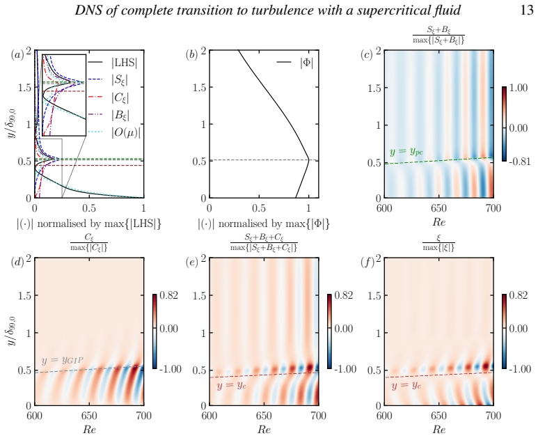
The load-bearing object is the Mode-II instability of a boundary layer at transcritical supercritical pressure: an inviscid mode tied to a minimum of kinematic viscosity at the pseudo-critical (Widom) line and to a generalised inflection point in the density-weighted velocity profile. In the linear stage it appears as two phase-locked, out-of-phase vorticity waves produced by shear and baroclinic effects; nonlinearly it produces billow roll-ups that periodically displace the Widom line, driving near-wall flow reversal and strong local shear layers. That shear-layer mechanism converts a single 2-D wave plus background noise into a full K-type breakdown, and the same flow then serves as a test case for variable-property turbulent scaling.
What would settle it
Run the same noise-initiated transcritical case with the solver's numerical noise reduced or reshaped, and with controlled broadband disturbances of measured amplitude injected instead; if transition moves downstream beyond the computational domain or does not occur when the noise amplitude is lowered, the claim that a single 2-D wave triggers transition by amplifying background noise is falsified.
Extended reading notes
Core claim
The central discovery is that Mode-II instability converts a single, moderate-amplitude two-dimensional disturbance into a complete laminar-to-turbulent transition, provided the wall temperature crosses the Widom line. The mechanism proceeds through a Kelvin-Helmholtz-like train of billows that displaces the Widom line, creating travelling near-wall flow reversals; these reversals generate localised shear layers that are inviscidly unstable, so three-dimensional modes grow from numerical background noise without any forced oblique wave. The resulting breakdown follows a fundamental (K-type) scenario with peak-valley splitting rather than the classic subharmonic H-type route. After transition, the turbulent boundary layer obeys semi-local variable-property scaling, and a variable-Prandtl enthalpy relation together with the Reynolds analogy gives a predictive estimate of skin friction and Stanton number.
Load-bearing premise
The transcritical breakdown claimed to start from background noise depends on the numerical noise floor in the DNS: its amplitude and spectral content are not quantified or matched to any physical disturbance environment, so the early transition could shift downstream or vanish under a different noise level.
Editorial extensions
If this is right
- Transition in transcritical supercritical boundary layers can be triggered by a single 2-D wave, with no need for controlled oblique-wave forcing.
- The natural path to turbulence is fundamental (K-type) breakdown, with aligned lambda-like vortices forming inside billow roll-ups rather than the staggered H-type pattern.
- Subharmonic H-type forcing still works, but it is delayed, and the resulting breakdown is driven by flow-reversal shear layers rather than classic secondary instability.
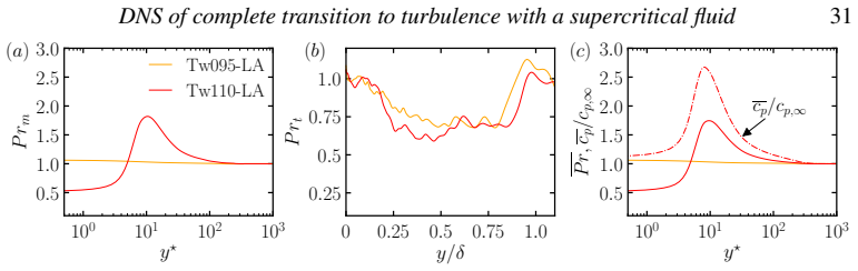
- The semi-local velocity transformation collapses the transcritical turbulent profiles, so variable-property scaling applies when density and viscosity fluctuations are moderate.
- Skin friction and heat transfer in the fully turbulent boundary layer can be estimated from the variable-Prandtl enthalpy relation combined with the Reynolds analogy, avoiding the need for costly DNS in engineering prediction.
Reading between the lines
- Because the early transition in the noise-initiated case is attributed to an unquantified numerical background noise floor, a testable extension would be to add controlled broadband noise of measured amplitude and spectrum and observe whether transition moves downstream or disappears.
- If the Mode-II mechanism is tied to a kinematic-viscosity minimum, so other non-polar supercritical fluids with the same property topology should exhibit the same single-wave transition route; this could be checked by linear stability analysis and DNS for fluids beyond the Van der Waals model used here.
- If the Reynolds analogy indeed holds across transcritical conditions, engineering heat-transfer correlations for supercritical heat exchangers and power cycles could be simplified substantially, though the present evidence is limited to one Reynolds number and one wall-temperature ratio.
- The travelling flow-reversal zones behave like unsteady separation bubbles, which suggests that experimental techniques developed for laminar separation bubbles, such as time-resolved wall-temperature or velocity imaging, could be adapted to detect this transition route in supercritical flows.
Editorial analysis
A structured set of objections, weighed in public.
Referee Report
Summary. The paper presents direct numerical simulations of laminar-to-turbulent transition in a heated zero-pressure-gradient flat-plate boundary layer with a fluid at supercritical pressure, comparing a liquid-like subcritical case (Tw095) with a transcritical case (Tw110) that crosses the pseudo-critical (Widom) line. The authors analyze the linear and nonlinear evolution of the newly identified Mode-II instability, show that nonlinear 2-D forcing produces billow-like structures and near-wall flow reversal, and examine 3-D breakdown with finite and infinitesimal oblique-wave forcing. They report a K-type breakdown triggered by numerical background noise in the Tw110-IA case and argue that a single 2-D wave can therefore promote transition in the transcritical regime. In the turbulent region, they show that the Patel-Trettel-Larsson velocity transformation collapses the profiles and develop an estimation model for skin friction and Stanton number based on van Driest's variable-Prandtl-number enthalpy relation.
Significance. If the main claims hold, this is a substantial contribution to the stability and transition literature for supercritical fluids. The paper provides the first complete DNS of transition with a highly non-ideal fluid, demonstrates the nonlinear consequences of Mode-II instability, identifies an APG-like breakdown mechanism caused by pseudo-boiling, and offers a practical heat-transfer estimation route. The work is strengthened by careful LST-DNS comparisons of eigenfunctions, growth rates, and phase speeds, a grid-resolution study for the transcritical case (Appendix A), detailed modal and structural analyses of K- and H-type routes, and publicly available source code for the engineering estimation model. The central transition pathway for finite-amplitude 3-D forcing is well supported by the DNS evidence. However, the stronger claim that transition can be triggered by a single 2-D wave amplifying background noise rests on a case whose noise floor is not quantified, and the engineering model is partly calibrated against the same DNS it is asked to predict.
major comments (3)
- [§5.1, Fig. 11(d), Table 2] The abstract and §7 claim that in the transcritical regime a single 2-D wave can 'strongly amplify background noise' and trigger transition. This claim rests on case Tw110-IA, where the 3-D forcing amplitude is A3-D = 1.0e-8 and the text states that mode (1,1) 'arises initially due to numerical background noise'. The amplitude and spectral content of that noise are never measured, and no controlled variation of the noise level or composition is reported. Because the spanwise domain is restricted to one fundamental wavelength and the grid-resolution study in Appendix A is performed for Tw110-LA rather than for Tw110-IA, the observed K-type breakdown could in principle be a grid, round-off, or scheme-dependent artifact. Quantifying the noise floor, preferably with a resolution study and a small-amplitude sweep of 3-D disturbances, is necessary before the 'transition from noise alone' pathway is established as a physical receptivity result.
- [§6.2, Eqs. (6.2)-(6.5), Figs. 21-25] The 'predictive model' for skin friction and heat transfer is presented as a tool, but its inputs include the DNS-computed mixed Prandtl number P r_m and the DNS-informed assumption P r_m ≈ P r. The Stanton number prediction is over-predicted by about 30% at R e_theta = 881, and the close agreement obtained via the Reynolds analogy uses C'_f from the same estimation. For a reader, it is unclear which quantities are truly predicted from free-stream and wall conditions alone and which are fitted or extracted from the DNS. Please state this limitation explicitly and distinguish the consistency-check nature of the comparison from a fully independent prediction.
- [Appendix A, Table 3] The grid-resolution sensitivity analysis is reported only for Tw110-LA, whose 3-D forcing is finite and large (A3-D = 8.5e-5). The case most sensitive to numerical background noise, Tw110-IA, has a 3-D forcing amplitude four orders of magnitude smaller, so a coarsening test for that case would be the relevant check for the central 'noise-amplification' claim. Without it, the robustness of the Tw110-IA breakdown to resolution and numerical scheme remains unverified.
minor comments (5)
- [§4.1, Eq. (4.1)] The typeset vorticity-perturbation equation contains stray markup symbols in the term annotations (e.g., '⌟⟨⟨⟪rl⟫⌟⟨l⟪2'), which obscure the definitions of S_xi, C_xi, and B_xi. Please re-typeset the equation and its labels.
- [§6.2, Fig. 23] The statement that Jensen's inequality implies 'χ ≠ χ(h,p)' is imprecise; the point is presumably that the Reynolds average of the thermophysical property evaluated at the Favre-averaged enthalpy differs from the property evaluated at the mean enthalpy due to fluctuation correlations. Please rephrase for clarity.
- [§4.2, Figs. 9, 15, and 17] The green shading used to indicate the Widom-line region is defined as 'between 98% max{c_p} and max{c_p}' in Fig. 9 but as 'between 95% max{c_p} and max{c_p}' in Figs. 15 and 17. Please make the threshold consistent and justify the choice.
- [§6.1, Fig. 20] The statement that the Patel et al. (2016) transformation 'collapses well the velocity profiles' should be rephrased as 'collapses the velocity profiles well' or similar, and the collapse should be quantified (e.g., maximum deviation from the log law) rather than stated qualitatively.
- [§3.2, Eq. (3.1)] The disturbance function f(x) is given without an indication of its peak value; stating that the integral or maximum of f(x) is normalized to unity would help the reader connect the specified A2-D and A3-D values to the actual forcing amplitude.
Circularity Check
No significant circularity: transition claims are DNS observations, and the §6 estimation model is a consistency check; minor self-citations are not load-bearing.
full rationale
The paper's central transition and breakdown findings are derived from direct numerical simulation and are not circular. Case Tw110-IA uses an infinitesimal 3-D forcing amplitude (A3-D = 1.0e-8, Table 2), and the authors state that mode (1,1) 'arises initially due to numerical background noise' (§5.1, Fig. 11d). This noise floor is not quantified or calibrated to a physical disturbance environment, which is a missing external support for the 'transition from noise alone' claim, but it is not a reduction of the result to its inputs: no parameter is fitted to the observed breakdown location, and the breakdown is observed rather than derived from the noise assumption. The §6 estimation model is a consistency check against the same DNS rather than a fitted prediction: the skin-friction prediction uses a Johnson-King/Coles mixing-length formulation with standard constants and the VdW/JST property models; the assumption Prm ≈ Pr is tested against the same DNS, and the Reynolds-analogy-based Stanton estimate uses the classical law s ≈ 1 as verified in Fig. 24, not a parameter fitted to the DNS Stanton number. Self-citations (e.g., Boldini et al. 2024a for K-type mode (0,1) dominance, and Bugeat et al. 2024 for the vorticity mechanism) support interpretation and context, but the load-bearing observations are made and compared within the present DNS/LST framework. No circular step meets the quote-and-reduction standard, so the score reflects only minor, non-load-bearing self-citations.
Assumptions & free parameters
assumptions (5)
- domain assumption The Van der Waals cubic equation of state with JST transport models accurately represents the relevant supercritical thermodynamics and transport for the instability and breakdown mechanisms.
- ad hoc to paper Numerical background noise in the DNS acts as a proxy for physical free-stream turbulence or other 3-D disturbances in the IA case.
- domain assumption The flow is two-dimensional in the mean, spanwise-periodic, and the initial boundary layer is a ZPG self-similar solution.
- standard math Stokes hypothesis (zero bulk viscosity) and Fourier's law of heat conduction hold for the supercritical fluid.
- domain assumption The recovery factor for the adiabatic wall enthalpy is r = Pr^(1/3) = 1.
Cite this review
Pith. "Pith review of Direct numerical simulation of complete transition to turbulence with a fluid at supercritical pressure." pith.science (2026). https://pith.science/paper/7QGMU2EI
@misc{pith2026250606703,
  author       = {Pith},
  title        = {Pith review of: Direct numerical simulation of complete transition to turbulence with a fluid at supercritical pressure},
  year         = {2026},
  howpublished = {\url{https://pith.science/paper/7QGMU2EI}},
  note         = {Machine review of arXiv:2506.06703}
}
abstract
The objective of this work is to investigate the unexplored laminar-to-turbulent transition of a heated flat-plate boundary layer with a fluid at supercritical pressure. Two temperature ranges are considered: a subcritical case, where the fluid remains entirely in the liquid-like regime, and a transcritical case, where the pseudo-critical (Widom) line is crossed and pseudo-boiling occurs. Fully compressible direct numerical simulations are used to study (i) the linear and nonlinear instabilities, (ii) the breakdown to turbulence, and (iii) the fully developed turbulent boundary layer. In the transcritical regime, two-dimensional forcing generates not only a train of billow-like structures around the Widom line, resembling Kelvin-Helmholtz instability, but also near-wall travelling regions of flow reversal. These spanwise-oriented billows dominate the early nonlinear stage. When high subharmonic three-dimensional forcing is applied, staggered $\Lambda$-vortices emerge more abruptly than in the subcritical case. However, unlike the classic H-type breakdown under zero pressure gradient observed in ideal-gas and subcritical regimes, the H-type breakdown is triggered by strong shear layers caused by flow reversals -- similar to that observed in adverse-pressure-gradient boundary layers. Without oblique wave forcing, transition is only slightly delayed and follows a naturally selected fundamental breakdown (K-type) scenario. Hence, in the transcritical regime, it is possible to trigger nonlinearities and achieve transition to turbulence relatively early using only a single two-dimensional wave that strongly amplifies background noise. In the fully turbulent region, we demonstrate that variable-property scaling accurately predicts turbulent skin-friction and heat-transfer coefficients.
Figures


Figures from the paper (26 more)






Reference graph
Works this paper leans on
-
[1]
, " * write output.state after.block = add.period write newline
ENTRY address author booktitle chapter edition editor howpublished institution journal key month note number organization pages publisher school series title type volume year eprint label extra.label sort.label short.list INTEGERS output.state before.all mid.sentence after.sentence after.block FUNCTION init.state.consts #0 'before.all := #1 'mid.sentence ...
-
[2]
write newline
" write newline "" before.all 'output.state := FUNCTION n.dashify 't := "" t empty not t #1 #1 substring "-" = t #1 #2 substring "--" = not "--" * t #2 global.max substring 't := t #1 #1 substring "-" = "-" * t #2 global.max substring 't := while if t #1 #1 substring * t #2 global.max substring 't := if while FUNCTION word.in bbl.in capitalize " " * FUNCT...
-
[3]
& Sandham, N
Alam, M. & Sandham, N. D. 2000 Direct numerical simulation of `short' laminar separation bubbles with turbulent reattachment . J. Fluid Mech. 410 , 1--28
2000
-
[4]
, Kloker, M
Babucke, A. , Kloker, M. & Rist, U. 2007 Direct numerical simulation of a serrated nozzle end for jet-noise reduction. In T ransactions of the H igh P erformance C omputing C enter, S tuttgart ( HLRS ) 2007\/ , p. 319–337
2007
-
[5]
Bae, J. H. , Yoo, J. Y. & Choi, H. 2005 Direct numerical simulation of turbulent supercritical flows with heat transfer . Phys. Fluids 17 , 105104
work page 2005
-
[6]
Bake, S. , Meyer, D. G. W. & Rist, U. 2002 Turbulence mechanism in K lebanoff transition: a quantitative comparison of experiment and direct numerical simulation . J. Fluid Mech. 459 , 217–243
work page 2002
-
[7]
Banuti, D. T. 2015 Crossing the W idom-line -- S upercritical pseudo-boiling . J. Supercrit. Fluids 98 , 12–16
work page 2015
-
[8]
Boldini, P. C. , Bugeat, B. , Peeters, J. W. R. , Kloker, M. & Pecnik, R. 2024 a\/ Direct numerical simulations of K -type transition in a flat-plate boundary layer with supercritical fluids, arXiv:arXiv: 2411.14286
work page Pith review arXiv 2024
Show all 84 references
-
[9]
Boldini, P. C. , Bugeat, B. , Peeters, J. W. R. , Kloker, M. & Pecnik, R. 2024 b\/ Transient growth in diabatic boundary layers with fluids at supercritical pressure . Phys. Rev. Fluids 9 , 083901
2024
-
[10]
Boldini, P. C. , Hirai, R. , Costa, P. , Peeters, J. W. R. & Pecnik, R. 2025 CUBENS : A GPU -accelerated high-order solver for wall-bounded flows with non-ideal fluids . Computer Physics Communications 309 , 109507
2025
-
[11]
, Boldini, P
Bugeat, B. , Boldini, P. C. , Hasan, A. M. & Pecnik, R. 2024 Instability in strongly stratified plane C ouette flow with application to supercritical fluids . J. Fluid Mech. 984 , A31
2024
-
[12]
, Boldini, P
Bugeat, B. , Boldini, P. C. & Pecnik, R. 2022 On the new unstable mode in the boundary layer flow of supercritical fluids. In Proceedings of the 12th International Symposium on Turbulence and Shear Flow Phenomena (TSFP-12)\/
2022
-
[13]
Candler, G. V. 2019 Rate effects in hypersonic flows . Annu. Rev. Fluid Mech. 51 , 379–402
2019
-
[14]
Cao, L. Y. , Xu, R. N. , Yan, J. J. , He, S. & Jiang, X. P. 2021 Direct numerical simulation of convective heat transfer of supercritical pressure CO2 in a vertical tube with buoyancy and thermal acceleration effect . J. Fluid Mech. 927 , A29
2021
-
[15]
Chang, C. L. & Malik, M. R. 1994 Oblique-mode breakdown and secondary instability in supersonic boundary layers . J. Fluid Mech. 273 , 323--360
1994
-
[16]
1956 The law of the wake in the turbulent boundary layer
Coles, D. 1956 The law of the wake in the turbulent boundary layer . J. Fluid Mech. 1 (2), 191--226
1956
-
[17]
Craik, D. D. A. 1971 Nonlinear resonant instability in boundary layers . J. Fluid Mech. 50 , 393413
1971
-
[18]
van Driest, E. R. 1951 Turbulent boundary layer in compressible fluids . J. Aeronaut. Sci. 18 , 145--160
1951
-
[19]
van Driest, E. R. 1955 The turbulent boundary layer with variable P randtl number. In 50 Jahre Grenzschichtforschung: Eine Festschrift in Originalbeiträgen\/ (ed. H. Görtler & W. Tollmien ) , p. 257–271 . Vieweg+Teubner Verlag
1955
-
[20]
& Martín, M
Duan, L. & Martín, M. P. 2011 Direct numerical simulation of hypersonic turbulent boundary layers. P art 4. E ffect of high enthalpy . J. Fluid Mech. 684 , 25--59
2011
-
[21]
Fasel, H. F. , Rist, U. & Konzelmann, U. 1990 Numerical investigation of the three-dimensional development in boundary-layer transition . AIAA J. 28 , 29–37
1990
-
[22]
2011 Transition and stability of high-speed boundary layers
Fedorov, A. 2011 Transition and stability of high-speed boundary layers . Annu. Rev. Fluid Mech. 43 , 79–95
2011
-
[23]
& Kloker, M
Fezer, A. & Kloker, M. 1999 Spatial direct numerical simulation of transition phenomena in supersonic flat-plate boundary layers. In Laminar–Turbulent Transition (ed. R. Kobayashi)\/ , p. 415–420 . Springer
1999
-
[24]
Franko, K. J. & Lele, S. K. 2013 Breakdown mechanisms and heat transfer overshoot in hypersonic zero pressure gradient boundary layers . J. Fluid Mech. 730 , 491--532
2013
-
[25]
, Bienner, A
Gloerfelt, X. , Bienner, A. & Cinnella, P. 2023 High-subsonic boundary-layer flows of an organic vapour . J. Fluid Mech. 971 , A8
2023
-
[26]
& Sahu, K
Govindarajan, R. & Sahu, K. C. 2014 Instabilities in viscosity-stratified flow . Annu. Rev. Fluid Mech. 46 , 331–353
2014
-
[27]
, Colonna, P
Guardone, A. , Colonna, P. , Pini, M. & Spinelli, A. 2024 Nonideal compressible fluid dynamics of dense vapors and supercritical fluids . Annu. Rev. Fluid Mech. 56 (1), 241--269
2024
-
[28]
, Yang, X
Guo, J. , Yang, X. I. A. & Ihme, M. 2022 Structure of the thermal boundary layer in turbulent channel flows at transcritical conditions . J. Fluid Mech. 934 , A45
2022
-
[29]
& Fasel, H
Hader, C. & Fasel, H. F. 2019 Direct numerical simulations of hypersonic boundary-layer transition for a flared cone: fundamental breakdown . J. Fluid Mech. 869 , 341--384
2019
-
[30]
Hasan, A. M. , Larsson, J. , Pirozzoli, S. & Pecnik, R. 2023 Incorporating intrinsic compressibility effects in velocity transformations for wall-bounded turbulent flows . Phys. Rev. Fluids 8 , L112601
2023
-
[31]
Hasan, A. M. , Larsson, J. , Pirozzoli, S. & Pecnik, R. 2024 Estimating mean profiles and fluxes in high-speed turbulent boundary layers using inner/outer-layer scalings . AIAA J. 62 (2), 848--853
2024
-
[32]
, Tian, R
He, J. , Tian, R. , Jiang, P. X. & He, S. 2021 Turbulence in a heated pipe at supercritical pressure . J. Fluid Mech. 920 , A45
2021
-
[33]
1988 Secondary instability of boundary layers
Herbert, T. 1988 Secondary instability of boundary layers . Annu. Rev. Fluid Mech. 20 , 487--526
1988
-
[34]
Johnson, D. A. & King, L. 1985 A mathematically simple turbulence closure model for attached and separated turbulent boundary layers . AIAA J. 23 (11), 1684--1692
1985
-
[35]
Jossi, A. J. , Stiel, L. I. & Thodos, G. 1962 The viscosity of pure substances in the dense gaseous and liquid phases . AIChE Jour. 8 , 59--63
1962
-
[36]
Kachanov, Yu. S. 1994 Physical mechanisms of laminar-boundary-layer transition . Annu. Rev. Fluid Mech. 26 , 411--482
1994
-
[37]
Kachanov, Yu. S. & Levchenko, V. Ya. 1984 The resonant interaction of disturbances at laminar-turbulent transition in a boundary layer . J. Fluid Mech. 138 , 209--247
1984
-
[38]
2019 Heated transcritical and unheated non-transcritical turbulent boundary layers at supercritical pressures
Kawai, S. 2019 Heated transcritical and unheated non-transcritical turbulent boundary layers at supercritical pressures . J. Fluid Mech. 865 , 563–601
2019
-
[39]
, Hickey, J.-P
Kim, K. , Hickey, J.-P. & Scalo, C. 2019 Pseudophase change effects in turbulent channel flow under transcritical temperature conditions . J. Fluid Mech. 871 , 52–91
2019
-
[40]
Klaassen, G. P. & Peltier, W. R. 1985 The onset of turbulence in finite-amplitude K elvin- H elmholtz billows . J. Fluid Mech. 155 , 1--35
1985
-
[41]
Klebanoff, P. S. , Tidstrom, K. D. & Sargent, L. M. 1962 The three-dimensional nature of boundary-layer instability . J. Fluid Mech. 12 , 1--34
1962
-
[42]
1993 Direkte numerische S imulation des laminar-turbulenten S trömungsumschlages in einer stark verzögerten G renzschicht
Kloker, M. 1993 Direkte numerische S imulation des laminar-turbulenten S trömungsumschlages in einer stark verzögerten G renzschicht . PhD thesis, University of Stuttgart
1993
-
[43]
2024 A note on the flow topology during laminar-turbulent transition induced by T ollmien- S chlichting waves
Kloker, M. 2024 A note on the flow topology during laminar-turbulent transition induced by T ollmien- S chlichting waves. ResearchGate, Report Number: IAG-TN-2024-LTT-02, available at: https://www.researchgate.net/publication/385746142
2024
-
[44]
& Fasel, H
Kloker, M. & Fasel, H. 1995 Direct numerical simulation of boundary-layer transition with strong adverse pressure gradient. In Laminar-Turbulent Transition\/ (ed. Ryoji Kobayashi ) , pp. 481--488 . Berlin, Heidelberg: Springer Berlin Heidelberg
1995
-
[45]
Kosorygin, V. S. 1994 Stability and transition to turbulence in 2-D boundary layer under the influence of adverse pressure gradients. In Nonlinear Instability of Nonparallel Flows\/ . IUTAM-Sym., Potsdam, USA, 1993
1994
-
[46]
& Kawai, S
Kuya, Y. & Kawai, S. 2021 High-order accurate kinetic-energy and entropy preserving (KEEP) schemes on curvilinear grids . J. Comput. Phys. 442 , 110482
2021
-
[47]
, Guo, J
Li, F. , Guo, J. , Bai, B. & Ihme, M. 2023 Analysis of real-fluid thermodynamic effects on turbulent statistics in transcritical channel flows . Phys. Rev. Fluids 8 , 024605
2023
-
[48]
, Zhang, W
Li, F. , Zhang, W. , Bai, B. & Ihme, M. 2024 Small-scale turbulent characteristics in transcritical wall-bounded flows . J. Fluid Mech. 986 , A36
2024
-
[49]
, Kaminski, A
Liu, C.-L. , Kaminski, A. & Smyth, W. D. 2023 The effects of boundary proximity on K elvin– H elmholtz instability and turbulence . J. Fluid Mech. 966 , A2
2023
-
[50]
, Sharma, A
Luhar, M. , Sharma, A. S. & McKeon, B. J. 2014 On the structure and origin of pressure fluctuations in wall turbulence: predictions based on the resolvent analysis . J. Fluid Mech. 751 , 38–70
2014
-
[51]
Ma, P. C. , Yang, X. I. A. & Ihme, M. 2018 Structure of wall-bounded flows at transcritical conditions . Phys. Rev. Fluids 3 , 034609
2018
-
[52]
2012 Analysis and optimization of numerical sponge layers as a nonreflective boundary treatment
Mani, A. 2012 Analysis and optimization of numerical sponge layers as a nonreflective boundary treatment . J. Comput. Phys. 231 , 704--716
2012
-
[53]
, Rist, U
Maucher, U. , Rist, U. , Kloker, M. & Wagner, S. 2000 DNS of laminar-turbulent transition in separation bubbles. In High Performance Computing in Science and Engineering ’99 (ed. E Krause, W. Jäger (Eds.))\/ , p. 279–294 . Springer-Verlag, Berlin
2000
-
[54]
Monkewitz, P. A. 1988 Subharmonic resonance, pairing and shredding in the mixing layer . J. Fluid Mech. 188 , 223--252
1988
-
[55]
, Bellan, J
Morellina, S. , Bellan, J. & Cutts, J. 2020 Global thermodynamic, transport-property and dynamic characteristics of the V enus lower atmosphere below the cloud layer . Icarus 350 , 113761
2020
-
[56]
Morkovin, M. V. 1969 On the many faces of transition. In Viscous Drag Reduction\/ (ed. C. S. Wells ) , p. 1–31 . Springer
1969
-
[57]
, Patel, A
Nemati, H. , Patel, A. , Boersma, B. J. & Pecnik, R. 2015 Mean statistics of a heated turbulent pipe flow at supercritical pressure . Int. J. Heat Mass Transf. 83 , 741--752
2015
-
[58]
, Patel, A
Nemati, H. , Patel, A. , Boersma, B. J. & Pecnik, R. 2016 The effect of thermal boundary conditions on forced convection heat transfer to fluids at supercritical pressure . J. Fluid Mech. 800 , 531–556
2016
-
[59]
Okong’o, N. A. & Bellan, J. 2002 Consistent boundary conditions for multicomponent real gas mixtures based on characteristic waves . J. Comput. Phys. 176 , 330--344
2002
-
[60]
, Boersma, B
Patel, A. , Boersma, B. J. & Pecnik, R. 2016 The influence of near-wall density and viscosity gradients on turbulence in channel flows . J. Fluid Mech. 809 , 793–820
2016
-
[61]
Peeters, J. W. R. , Pecnik, R. , Rohde, M. , van der Hagen, T. H. J. J. & Boersma, B. J. 2016 Turbulence attenuation in simultaneously heated and cooled annular flows at supercritical pressure . J. Fluid Mech. 799 , 505–540
2016
-
[62]
& Kloker, M
Ren, J. & Kloker, M. 2022 Instabilities in three-dimensional boundary-layer flows with a highly non-ideal fluid . J. Fluid Mech. 951 , A9
2022
-
[63]
, Marxen, O
Ren, J. , Marxen, O. & Pecnik, R. 2019 Boundary-layer stability of supercritical fluids in the vicinity of the W idom line . J. Fluid Mech. 871 , 831–864
2019
-
[64]
& Fasel, H
Rist, U. & Fasel, H. 1995 Direct numerical simulation of controlled transition in a flat-plate boundary layer . J. Fluid Mech. 298 , 211–248
1995
-
[65]
& Gloerfelt, X
Robinet, J.-C. & Gloerfelt, X. 2019 Instabilities in non-ideal fluids . J. Fluid Mech. 880 , 1–4
2019
-
[66]
Saric, W. S. , Reed, H. L. & Kerschen, E. J. 2002 Boundary-layer receptivity to freestream disturbances . Annu. Rev. Fluid Mech. 34 , 291–319
2002
-
[67]
, Hamman, C
Sayadi, T. , Hamman, C. & Moin, P. 2013 Direct numerical simulation of complete H -type and K -type transitions with implications for the dynamics of turbulent boundary layers . J. Fluid Mech. 724 , 480–509
2013
-
[68]
Schmid, P. J. & Henningson, D. S. 2001 Stability and transition in shear flows\/ . Springer
2001
-
[69]
, Cinnella, P
Sciacovelli, L. , Cinnella, P. & Gloerfelt, X. 2017a Direct numerical simulations of supersonic turbulent channel flows of dense gases . J. Fluid Mech. 821 , 153--199
-
[70]
, Gloerfelt, X
Sciacovelli, L. , Gloerfelt, X. , Passiatore, D. , Cinnella, P. & Grasso, F. 2020 Numerical investigation of high-speed turbulent boundary layers of dense gases . Flow Turbul. Combust. 105 , 555--579
2020
-
[71]
, Kuya, Y
Shima, N. , Kuya, Y. , Tamaki, Y. & Kawai, S. 2021 Preventing spurious pressure oscillations in split convective form discretization for compressible flows . J. Comput. Phys. 427 , 110060
2021
-
[72]
& Fasel, H
Sivasubramanian, J. & Fasel, H. F. 2015 Direct numerical simulation of transition in a sharp cone boundary layer at M ach 6: fundamental breakdown . J. Fluid Mech. 768 , 175--128
2015
-
[73]
Smits, A. J. & Dussauge, J.-P. 2006 Turbulent Shear Layers in Supersonic Flow\/ . Springer Science & Business Media
2006
-
[74]
Stiel, L. I. & Thodos, G. 1964 The thermal conductivity of nonpolar substances in the dense gaseous and liquid regions . AIChE Jour. 10 , 26--30
1964
-
[75]
Taylor, G. I. 1936 Statistical theory of turbulence. P art V . E ffect of turbulence on boundary layer. T heoretical discussion of relationship between scale of turbulence and critical resistance of spheres . Proc. R. Soc. Lond. A. 156 , 307--317
1936
-
[76]
& Larsson, J
Trettel, A. & Larsson, J. 2016 Mean velocity scaling for compressible wall turbulence with heat transfer . Phys. Fluids 28 (2), 026102
2016
-
[77]
& Gaitonde, D
Unnikrishnan, S. & Gaitonde, D. V. 2020 Linear, nonlinear and transitional regimes of second-mode instability . J. Fluid Mech. 905 , A25
2020
-
[78]
Van der Waals , J. D. 1873 Over de continuiteit van den gas- en vloeistoftoestand . PhD thesis, Hoogeschool te Leiden
-
[79]
1969 Boundary Layers of Flow and Temperature\/
Walz, A. 1969 Boundary Layers of Flow and Temperature\/ . MIT Press, Cambridge
1969
-
[80]
& Yang, V
Wang, X. & Yang, V. 2017 Supercritical mixing and combustion of liquid-oxygen/kerosene bi-swirl injectors . J. Propul. Power 33 , 316–322
2017
-
[81]
, Gibis, T
Wenzel, C. , Gibis, T. , Kloker, M. & Rist, U. 2021 Reynolds analogy factor in self-similar compressible turbulent boundary layers with pressure gradients . J. Fluid Mech. 907 , R4
2021
-
[82]
White, F. M. 2006 Viscous Fluid Flow, 3rd Edition\/ . Boston: McGraw-Hill
2006
-
[83]
Yoo, J. Y. 2013 The turbulent flows of supercritical fluids with heat transfer . Annu. Rev. Fluid Mech. 45 , 495–525
2013
-
[84]
1998 High-order finite-difference schemes for numerical simulation of hypersonic boundary-layer transition
Zhong, X. 1998 High-order finite-difference schemes for numerical simulation of hypersonic boundary-layer transition . J. Comput. Phys. 144 (2), 662--709
1998
Reviewed August 7, 2026 · model on record in the stance chip above.
Discussion (0). Sign in to comment.