Understanding Sharpness Dynamics in NN Training with a Minimalist Example: The Effects of Dataset Difficulty, Depth, Stochasticity, and More

Chulhee Yun; Geonhui Yoo; Minhak Song

REVIEW 3 major objections 4 minor 15 references

Understanding Sharpness Dynamics in NN Training with a Minimalist Example: The Effects of Dataset Difficulty, Depth, Stochasticity, and More

T0 review · 3 major / 4 minor · reviewed 2026-08-07 · deepseek-v4-flash

Challenge this review Re-run · record.json Download PDF Read on arXiv ↗

Pith's one-line read Sharpness at the final minimum is governed by a data-only quantity Q and a conserved layer imbalance.

desk verdict A solid, genuinely new minimalist analysis of progressive sharpening that deserves peer review; the main caveat is an unproved convergence assumption and a missing disclosure of failed runs. read the letter →

arxiv 2506.06940 v1 pith:NNIIV3DM submitted 2025-06-07 cs.LG

Geonhui Yoo , Minhak Song , Chulhee Yun This is my paper

classification cs.LG

keywords progressivesharpeningedgeofstabilitysharpnessdeeplinearnetworksdatasetdifficultylayerimbalancegradientflowstochasticdescent

verification ladder T0 review T1 audit T2 compute T3 formal

The pith

A machine-rendered reading of the paper's core claim, the machinery that carries it, and where it could break.

The reading

This paper tries to explain progressive sharpening — the tendency of the loss landscape's sharpness to rise during gradient training and then hover near the stability limit $2/\eta$ — using a deliberately minimal model: a deep linear network with a single neuron per layer. The paper shows that in this model the sharpness at a zero-error solution is pinned down by two quantities: the dataset difficulty $Q$, a sum over data directions of label energy divided by squared singular value, and the layer imbalance $C$, a measure of how weight norm is split across layers. Because gradient flow conserves $C$, the final sharpness of full-batch training can be predicted from the data and the initialization alone, and the paper proves bounds whose dominant term is the predicted sharpness $\hat{S}_D=\sigma_1^2 Q^{(D-1)/D}/N$. The paper then reports that this data-only prediction correlates strongly with post-training sharpness in much wider, nonlinear networks on CIFAR-10, SVHN, and Google Speech Commands, and that SGD's batch size and step size act through the same $C$ mechanism. If the paper is right, a puzzling empirical phenomenon becomes a computable, data-dependent quantity with implications for learning-rate choice and initialization.

What carries the argument

The machinery has five parts. (1) The minimalist model $f(x;\theta)=(x^\top u)\prod_{i=1}^{D-1} v_i$, a deep linear network whose single neuron per layer makes the residual decompose exactly along the singular directions of the data matrix $X=\sum_i \sigma_i e_i w_i^\top$. (2) The dataset difficulty $Q=\sum_i d_i^2/\sigma_i^2$, a data-only scalar that measures how much weight the labels put on each direction relative to the data's energy in that direction. (3) The layer imbalance $C=\|\Pi_W u\|^2-v_1^2$ for $D=2$, the conserved quantity under gradient flow that also serves as the state variable for one GD/SGD step; the deep case replaces it with the balancedness condition $\|\Pi_W u\|=|v_1|=\cdots=|v_{D-1}|$. (4) The identity that at a zero-loss point the loss Hessian equals $(1/N)J^\top J$, the normalized Gauss-Newton / neural tangent kernel matrix, so sharpness becomes the spectral norm of a matrix written purely in terms of $\sigma_i$, $d_i$, and $C$. (5) The predicted sharpness $\hat{S}_D=\sigma_1^2 Q^{(D-1)/D}/N$, the numerically dominant bound term that the experiments compare with final sharpness in wider nonlinear networks. Theorem 5.9's explicit one-step formulas for the increase of $C$ under GD and SGD carry the batch-size and step-size conclusions.

What would settle it

Run gradient flow to zero loss on fixed two-label datasets whose measured $Q$ spans at least two orders of magnitude, using balanced initializations, and plot final sharpness against $Q$ on log-log axes; the theory predicts a slope of $(D-1)/D$ and a sign change in the depth-versus-sharpness slope exactly where $Q$ crosses 1, so a systematic deviation in either would falsify the depth and difficulty claims.

Watch

Extended reading notes

Core claim

The paper's central claim is that progressive sharpening — the rise of the loss Hessian's largest eigenvalue during training, up to the $2/\eta$ edge of stability — is governed in a tractable way by two quantities in its minimalist deep linear network with a single neuron per layer. It defines the dataset difficulty $Q=\sum_i d_i^2/\sigma_i^2$ using the singular-value decomposition of the training data and the label's expansion in the left singular basis, and the layer imbalance $C=\|\Pi_W u\|^2-v_1^2$ between the first layer's projected norm and the scalar second-layer weight. Theorems 4.3 and 4.6 prove that at any zero-loss minimizer the sharpness is trapped between bounds that grow with $Q$ and the leading singular value $\sigma_1$, shrink with $C$, and for balanced depth-$D$ networks are dominated by $\hat{S}_D=\sigma_1^2 Q^{(D-1)/D}/N$. Because gradient flow conserves $C$ and preserves balancedness, the full-batch convergence sharpness is fixed by the initialization and the data alone. The paper reports correlations between $\hat{S}_D$ and measured final sharpness of 0.81–0.99 for fully connected networks up to width 2048 with linear and nonlinear activations across CIFAR-10, SVHN, and Google Speech Commands, and proves for SGD that smaller batches and larger step sizes raise $C$ faster per update, which lowers the eventual sharpness. The same model also reproduces the oscillatory edge-of-stability regime, including loss spikes whose precise behavior depends on numerical precision.

Load-bearing premise

The load-bearing premise is that gradient flow actually converges to a global minimum with zero training error; if it stalls at a higher-error critical point, the sharpness bounds describe a minimizer the trajectory never visits, and the deep-network version of the claim additionally assumes layer norms start balanced, whereas the real-network experiments use default PyTorch initialization.

Editorial extensions

If this is right

Because $Q$ is computable from the data before training, $\hat{S}_D$ gives a training-free estimate of where full-batch gradient flow will end up, and through the $2/\eta$ rule it predicts whether a chosen learning rate will push GD into the edge of stability.
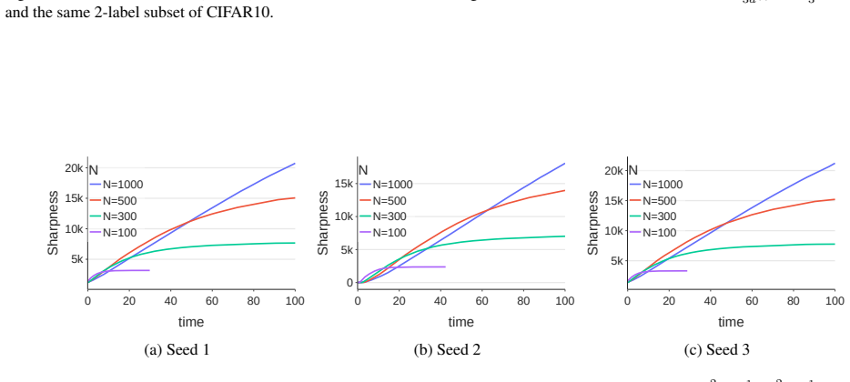
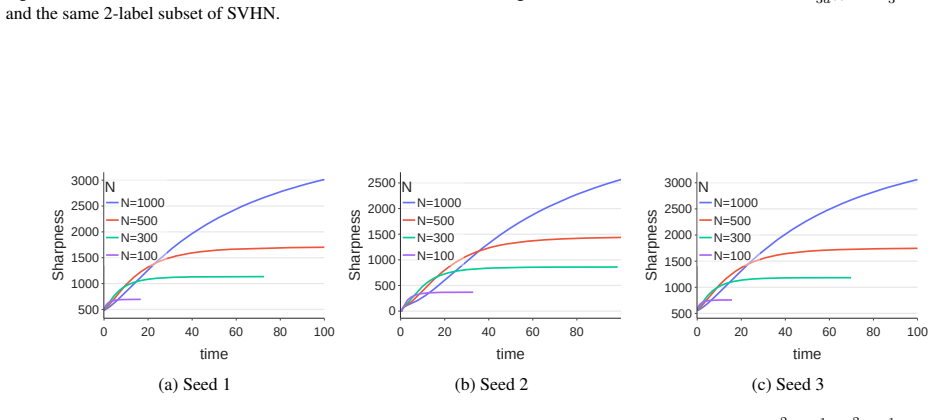
Depth is not intrinsically sharpening: for datasets with $Q>1$ deeper networks train to sharper minima, while for $Q<1$ adding depth flattens them; the paper verifies this flip for CIFAR-10 at $N=100$ versus $N=300$.
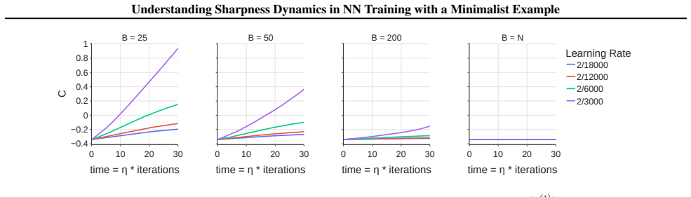
Batch size and learning rate act through one channel: smaller batches and larger steps increase the layer imbalance more per update, which reduces progressive sharpening, matching the empirical Phenomenon 1.
Since layer imbalance is conserved under gradient flow, the final sharpness of full-batch training is set at initialization, so two runs with different $C$ but the same data should land at different sharpness values.
The same minimalist model reproduces edge-of-stability oscillations, loss spikes, and a precision-dependent sharpness drop, making it a tractable testbed for mechanisms that also operate in Transformers.

Reading between the lines

Editorial extensions of the paper, not claims the author makes directly.

My inference: $Q$ is essentially the squared norm of the minimum-norm linear fit measured in units of the data's singular spectrum, so the paper's results connect progressive sharpening to how hard the dataset is to fit with small weights; this bridges to implicit-bias results in linear networks that the paper does not invoke.
My inference: the conservation law for $C$ suggests initialization is a direct handle on final sharpness — schemes that deliberately unbalance layer norms should move convergence sharpness up or down within the proved bounds — and this is testable in real networks beyond the paper's default-initialization experiments.
My inference: because the paper shows the sharpness drop at the edge of stability depends on machine precision and can even blow up at high precision, the widely observed stabilizing plateau may be partly a finite-precision artifact; the paper documents the phenomenon but does not draw this general conclusion.
My inference: the $Q<1$ versus $Q>1$ switch predicts a sharp transition in how depth affects minima as the training set grows, so sweeping $N$ finely around the $Q\approx 1$ point on a single dataset would give a crisp, quantitative test of the theory outside the minimalist model.

Share X Bluesky LinkedIn Reddit HN

Editorial analysis

A structured set of objections, weighed in public.

Desk editor's note, referee report, and a circularity audit.

Desk Editor's Note

read the letter

Short version: this paper deserves a serious referee and, in my view, acceptance after minor revisions. The core contribution is real: for a deep linear network with one neuron per layer but a general data matrix and labels, the authors derive two-sided bounds on sharpness at zero-loss minimizers in terms of a data-only quantity Q and the layer imbalance C. That is a genuine step beyond the scalar-network analyses of Zhu et al. and Kreisler et al., and beyond Marion and Chizat's upper bound for deep linear nets. The dominant term sigma_1^2/N * Q^((D-1)/D) is parameter-free, and the correlation check against final sharpness in wide nonlinear networks across three datasets is a legitimate out-of-sample prediction using 50 held-out dataset draws. The GD/SGD layer-imbalance theorem is also new, and the paper is appropriately careful about what it does and doesn't prove.

The main soft spot is Assumption 5.1: gradient flow converges to a zero-loss minimizer. Non-global critical points do exist in this model, so the bounds describe a minimizer the trajectory might not reach. The authors state the assumption explicitly, but the empirical validation only reports that runs were terminated when L < 1e-6; they never say how many random seeds, if any, failed to reach that threshold. If failed runs were dropped, the reported correlations are conditional on convergence, which should be disclosed. This is a fixable reporting gap, not a fatal flaw, and the stress-test note lands.

Two smaller items. The deep theory assumes balanced initialization, while the real-network validation uses default PyTorch init; the authors acknowledge this, and the correlations still hold, which is encouraging, but the depth prediction is tested outside its stated regime. There is also a subscript typo in Appendix B.3 (sigma_1^2 in a sum that should be sigma_i^2); the final result is correct, so this is cosmetic.

Who this is for: anyone working on edge-of-stability, progressive sharpening, or learning-rate schedules. The Q quantity will likely be reused. My recommendation: accept after minor revision, and ask the authors to report convergence failure rates and fix the typo.

Referee Report

3 major / 4 minor

Summary. The paper proposes a deep linear network with a single neuron per layer as a minimalist testbed for progressive sharpening and edge-of-stability behavior. It introduces a data-dependent quantity Q (dataset difficulty), derives lower and upper bounds on sharpness at zero-loss minimizers as functions of Q, depth, and layer imbalance (Theorems 4.3 and 4.6), and defines the predicted sharpness S_Dhat = σ1^2/N * Q^{(D-1)/D}. Under gradient flow, the layer imbalance is conserved (Lemma 5.2), so the convergence-sharpness bounds are determined by initialization (Corollaries 5.3 and 5.4). The paper also analyzes initial and convergence sharpness under αβ initialization (Theorems 5.6 and 5.7) and characterizes one-step changes of layer imbalance under GD and SGD (Theorem 5.9). Empirically, the minimalist model reproduces the dataset-size, depth, batch-size, and learning-rate trends of Phenomenon 1 and the edge-of-stability loss spikes; the predicted sharpness S_Dhat correlates with final sharpness in wider nonlinear networks on CIFAR-10, SVHN, and Google Speech Commands.

Significance. If the results hold, the paper supplies one of the cleanest available theoretical explanations for how data, depth, stochasticity, and step size control progressive sharpening. The main algebraic derivations are self-contained and appear correct; the definition of Q is data-only and the dominant term S_Dhat is not fitted to observed sharpness, so the correlation experiments (including 50 held-out dataset draws per setting) provide a meaningful, falsifiable check. The paper is also candid about the precision-dependence of edge-of-stability dynamics in Appendix D and about the preliminary nature of the nonlinear extension in Appendix E. The principal risks are that Assumption 5.1 (convergence of gradient flow to a zero-loss global minimum) is unverified in the empirical validation and that the deep-network prediction is tested with default PyTorch initialization while the theory assumes balanced layers.

major comments (3)

[Section 5.1, Assumption 5.1] Assumption 5.1 is load-bearing for Corollaries 5.3 and 5.4 and for Theorem 5.7: the sharpness bounds are for a zero-loss minimizer, but the trajectory may in principle converge to a non-global critical point, which does exist in this model (e.g., layer products equal to zero with the first-layer weight orthogonal to X^T y). The empirical validation in Section 5.1 sidesteps this by terminating runs at L(theta(t)) < 1e-6 and treating that iterate as theta(infinity), but the paper never reports how many of the 50 random seeds per setting failed to reach that threshold or what the sharpness values were for failed runs. If failed runs were excluded, the correlations in Figure 7 and Tables 5-7 are conditional on successful convergence, which materially changes the claim. Please report per-setting convergence counts, or prove within the minimalist model that gradient flow avoids non-global critical points.
[Section 4.2 and Section 5.1] The deep-network bounds in Theorem 4.6 and the predicted sharpness S_Dhat are derived under Assumption 4.5 that layers are balanced, and the gradient-flow analysis uses balanced initialization to preserve that property. However, the empirical validation in Section 5.1 (Figure 7, Figure 8, Tables 5-7) uses default PyTorch initialization, which is not balanced. The paper acknowledges the mismatch in a footnote, but still uses these experiments as evidence for the depth dependence Q^{(D-1)/D}. To make the depth claim load-bearing, the authors should either run the validation with balanced initialization or provide a quantitative argument that imbalance does not change the dominant scaling in the predicted sharpness.
[Section 5.2, Theorem 5.9] Theorem 5.9 shows that a single GD step increases C when C <= Omega_1/Psi_1 and that SGD increases C even more under an analogous condition, but it does not establish that the final value of C at convergence is ordered accordingly, nor that the final sharpness is ordered. The paper explicitly acknowledges this, so the theorem is not internally inconsistent; however, the ensuing qualitative claims about batch size and learning rate would be strengthened by a convergence-level statement or by evidence that the threshold conditions are satisfied along the entire trajectory, beyond the plotted points in Figures 21 and 22.

minor comments (4)

[Appendix B.3, proof of Theorem 4.6] In the upper-bound chain, the line containing \sum_{i=1}^r \sigma_1^2(o_i^*)^2 should read \sum_{i=1}^r \sigma_i^2(o_i^*)^2; the displayed equality is only correct after this substitution.
[Throughout] Several cross-references are mislabeled: Theorem 4.5 should be Assumption 4.5, Theorem 5.1 and Theorem 5.5 should be Assumption 5.1 and Assumption 5.5, Theorem 5.2 should be Lemma 5.2, and Theorem B.1 and Theorem B.3 should be Lemma B.1 and Lemma B.3. These do not affect the mathematics but should be corrected before publication.
[Section 5.1, Tables 5-7] The correlation values for tanh, SiLU, and ELU activations vary from about 0.6 to 0.9 across widths and depths, and the paper does not report confidence intervals or p-values. Reporting these would clarify which architecture regimes the predicted-sharpness correlation is robust in.
[Section 3.2 and Appendix D] The observation that edge-of-stability behavior is precision-dependent is interesting and appropriately reported, but the main text should mention this limitation earlier, since Figure 6 is presented as representative behavior of the model without noting the strong dependence on floating-point precision.

Circularity Check

0 steps flagged · score 0.0 of 10

No circularity: the sharpness bounds are derived algebraically from Q and the layer imbalance, and the predicted-sharpness proxy is not fitted to empirical sharpness.

full rationale

Q is defined from data only (Definition 4.1) and enters the minimizer equations through the zero-residual identity o_i = d_i/(sigma_i times the product of the v's), so the dependence of S(theta*) on Q is a mathematical consequence rather than an input. Theorem 4.3 and Theorem 4.6 derive two-sided bounds; the 'predicted sharpness' S_Dhat is the dominant term of those bounds, selected after the fact as a useful proxy, not calibrated to match observed sharpness. The empirical validation in Section 5.1 correlates S_Dhat with final sharpness across 50 random dataset draws and reports raw correlations without fitting a scale, so the correlation claim has independent content. Assumption 5.1 (GF converges to a global minimum) is an explicit convergence condition inherited by Corollaries 5.3, 5.4, and Theorem 5.7; it is a substantive assumption that could fail for non-global critical points, but it is not circular because it is not derived from or equivalent to the target sharpness bounds. The GD/SGD explanation in Theorem 5.9 relies on the empirically observed inequalities C <= T1 and C <= T2 rather than a proof that they hold throughout training; the paper explicitly acknowledges this as incomplete ('the theorem does not fully prove'), which is a gap in the argument, not a circular reduction. Self-citations such as Song & Yun (2023) appear only in related-work discussion and are not load-bearing for the paper's central derivations. Overall, no step reduces a prediction to its own inputs by construction.

Assumptions & free parameters 1 free parameters · 4 assumptions · 0 invented entities

The paper does not postulate new physical entities. Dataset difficulty Q and layer imbalance C are derived algebraic quantities, not fitted parameters or invented degrees of freedom. The main explicit premises are convergence of gradient flow, balancedness for deep networks, and the alpha-beta initialization scale, all stated in the text.

free parameters (1)

alpha^2, beta^2 (initialization variances) = alpha^2 = 1/(3d), beta^2 = 1/3 in experiments
Introduced in Assumption 5.5 as the scale of Gaussian initialization. They enter the expected sharpness bounds in Theorems 5.6 and 5.7, and in experiments they are set to match PyTorch default initialization rather than fitted to sharpness values.

assumptions (4)

domain assumption Assumption 5.1: gradient flow converges to a global minimum with L(theta(infinity))=0.
Used by Corollaries 5.3, 5.4, and Theorem 5.7 to identify the trajectory endpoint with a zero-loss minimizer. Not proved in the paper, but it is explicitly stated and is plausible for deep linear networks with squared loss.
domain assumption Assumption 4.5: balanced layers, i.e. ||Pi_W u|| = |v_1| = ... = |v_{D-1}|.
Needed for the arbitrary-depth sharpness bounds in Theorem 4.6 and Corollary 5.4. Balancedness is preserved by gradient flow under balanced initialization, but practical validation does not use balanced initialization.
domain assumption Assumption E.1: orthogonal data, i.e. XX^T is diagonal, for the nonlinear extension.
Introduced only in the preliminary nonlinear analysis of Appendix E to make the reparameterization exact. Not used for the main linear-model results.
standard math y is assumed to lie in col(X) for the zero-loss analysis; the paper argues this is without loss of generality via decomposition.
The orthogonal label component only adds a constant to the loss and, since the residual is orthogonal to col(X), the second-order residual term vanishes at the minimizer. This is a valid reduction rather than a hidden assumption.

how reviews work

0 comments

Cite this review

Pith. "Pith review of Understanding Sharpness Dynamics in NN Training with a Minimalist Example: The Effects of Dataset Difficulty, Depth, Stochasticity, and More." pith.science (2026). https://pith.science/paper/NNIIV3DM

@misc{pith2026250606940,
  author       = {Pith},
  title        = {Pith review of: Understanding Sharpness Dynamics in NN Training with a Minimalist Example: The Effects of Dataset Difficulty, Depth, Stochasticity, and More},
  year         = {2026},
  howpublished = {\url{https://pith.science/paper/NNIIV3DM}},
  note         = {Machine review of arXiv:2506.06940}
}

read the original abstract

When training deep neural networks with gradient descent, sharpness often increases -- a phenomenon known as progressive sharpening -- before saturating at the edge of stability. Although commonly observed in practice, the underlying mechanisms behind progressive sharpening remain poorly understood. In this work, we study this phenomenon using a minimalist model: a deep linear network with a single neuron per layer. We show that this simple model effectively captures the sharpness dynamics observed in recent empirical studies, offering a simple testbed to better understand neural network training. Moreover, we theoretically analyze how dataset properties, network depth, stochasticity of optimizers, and step size affect the degree of progressive sharpening in the minimalist model. We then empirically demonstrate how these theoretical insights extend to practical scenarios. This study offers a deeper understanding of sharpness dynamics in neural network training, highlighting the interplay between depth, training data, and optimizers.

Figures

Figures reproduced from arXiv: 2506.06940 by the authors.

**Figure 1.** GF closely tracks GD dynamics before EoS. Sharpness of GF saturates as loss converges to zero. Sharpness of GD saturates as it enters the EoS regime. For experimental details, refer to Section C.1. sharpening depends on problem parameters, based on the observations of Cohen et al. (2021). Their experiments examine the influence of factors such as network architecture and training data on the degree of progressive s… view at source ↗

**Figure 2.** Effect of dataset size, network depth, and network width of tanh NN, for experimental details, refer to Section C.1. 0 20 40 60 80 100 80 100 120 140 160 180 200 220 0 20 40 60 80 100 0 20 40 60 80 100 0 20 40 60 80 100 Learning Rate η=2/1000 η=2/800 η=2/600 η=2/400 η=2/200 time = η * iterations time = η * iterations time = η * iterations time = η * iterations Sharpness B = 125 B = 250 B = 500 B=N [PITH_FULL_IMAGE:… view at source ↗

**Figure 3.** Effect of batch size, and learning rate in SGD and GD, for experimental details, refer to Section C.1. • Batch size: Progressive sharpening occurs to a greater degree as the SGD batch size increases. When training with SGD, larger batch sizes lead to more pronounced progressive sharpening (see [PITH_FULL_IMAGE:figures/full_fig_p003_3.png] view at source ↗

Figures from the paper (26 more)

**Figure 4.** Figure 4: Effect of batch size and learning rate in our minimalist model (D = 2). We use a 2-label subset of N = 1000 from CIFAR10. 0 5 10 15 20 25 30 0 2k 4k 6k 8k 10k 12k 14k 16k N D=5 D=4 D=3 time Sharpness (a) Depth 0 100 200 300 400 0 1000 2000 3000 4000 5000 N N=1000 N=500…

**Figure 5.** Figure 5: Effects of depth and dataset size in minimalist models. All experiments used a 2-label subset of N = 1000 from CIFAR10. In (b), except for N = 1000, runs terminated after L(θ) < 10−7 . Optimizers. We consider three optimization algorithms: • Gradient Flow (GF): ˙θ(t) =…

**Figure 6.** Figure 6: Our model captures typical “edge of stability” behaviors. sharpness reaches 2/η, and then the sharpness oscillates around the threshold 2/η. Figure 6c and Figure 6d show the loss curve for the two models. As usually seen in the loss curves of practical models, the loss…

**Figure 8.** Figure 8: Depth vs Sharpness plot. “I” denotes identity activation, “T” denotes tanh activation, and “w” means width. experiments on SVHN and Google speech commands; see Section C.6. Based on [PITH_FULL_IMAGE:figures/full_fig_p008_8.png]

**Figure 9.** Figure 9: Effect of batch size and learning rate in minimal models in the dynamics of layer imbalance C(θ (t) ), in D = 2 & N = 1000. By Theorem 4.3, knowing C(θ ⋆ ) at convergence determines the bound of sharpness. Therefore, we focus on the change of C after an update of GD an…

**Figure 10.** Figure 10: Effect of dataset size, network depth, and network width of tanh NN, SVHN dataset 0 50 100 150 200 400 600 800 1000 1200 1400 1600 1800 0 50 100 150 0 50 100 150 0 50 100 150 Learning Rate η=2/8000.0 η=2/4000.0 η=2/2000.0 η=2/1500.0 η=2/1000.0 time = η * iterations ti…

**Figure 11.** Figure 11: Effect of batch size, and learning rate in SGD and GD of tanh NN, SVHN dataset. 0 50 100 0 5k 10k 15k 20k 0 50 100 0 50 100 0 50 100 Learning Rate η=2/15000 η=2/20000 η=2/25000 η=2/30000 η=2/40000 time = η * iterations time = η * iterations time = η * iterations time …

**Figure 12.** Figure 12: Effect of batch size, and learning rate in SGD and GD of minimal model, SVHN dataset. 0 20 40 60 80 100 0 5k 10k 15k 20k N N=1000 N=500 N=300 N=100 time Sharpness (a) Dataset size 0 20 40 60 80 100 0 50k 100k 150k 200k 250k D D=5 D=4 D=3 time Sharpness (b) Network dep…

**Figure 13.** Figure 13: Effect of dataset size, network depth of minimal model, SVHN dataset 28 [PITH_FULL_IMAGE:figures/full_fig_p028_13.png]

**Figure 14.** Figure 14: Effect of dataset size, network depth, and network width of tanh NN, Google speech commands dataset 0 50 100 150 100 110 120 130 140 150 160 170 180 0 50 100 150 0 50 100 150 0 50 100 150 Learning Rate η=2/800.0 η=2/600.0 η=2/400.0 η=2/200.0 η=2/150.0 time = η * itera…

**Figure 15.** Figure 15: Effect of batch size, and learning rate in SGD and GD of tanh NN, Google speech commands dataset 0 10 20 30 600 800 1000 1200 1400 1600 0 10 20 30 0 10 20 30 0 10 20 30 Learning Rate η=2/1500 η=2/2000 η=2/3000 η=2/4000 η=2/6000 time = η * iterations time = η * iterati…

**Figure 16.** Figure 16: Effect of batch size, and learning rate in SGD and GD of minimal model, 2-label subsets of Google speech commands dataset (yes vs no) 0 50 100 150 200 500 1000 1500 2000 2500 3000 3500 N N=1000 N=500 N=300 N=100 time Sharpness (a) Dataset size 0 20 40 60 80 100 120 14…

**Figure 17.** Figure 17: Effect of dataset size, network depth of minimal model, 2-label subsets of google speech commands dataset (yes vs no) 29 [PITH_FULL_IMAGE:figures/full_fig_p029_17.png]

**Figure 18.** Figure 18: Minimalist model (D = 2) trained on different random weight seed, normal distribution with α 2 = 1 3d , β2 = 1 3 initialized, and the same 2-label subset of CIFAR10. 0 20 40 60 80 100 5k 10k 15k 20k N N=1000 N=500 N=300 N=100 time Sharpness (a) Seed 1 0 20 40 60 80 10…

**Figure 19.** Figure 19: Minimalist model (D = 2) trained on different random weight seed, normal distribution with α 2 = 1 3d , β2 = 1 3 initialized, and the same 2-label subset of SVHN. 0 20 40 60 80 100 500 1000 1500 2000 2500 3000 N N=1000 N=500 N=300 N=100 time Sharpness (a) Seed 1 0 20 …

**Figure 20.** Figure 20: Minimalist model (D = 2) trained on different random weight seed, normal distribution with α 2 = 1 3d , β2 = 1 3 initialized, and the same 2-label subset of Google speech commands. 35 [PITH_FULL_IMAGE:figures/full_fig_p035_20.png]

**Figure 21.** Figure 21: Change of T1 0 5 10 15 20 25 30 0 0.5 1 1.5 2 2.5 3 3.5 4 0 5 10 15 20 25 30 0 5 10 15 20 25 30 Learning Rate 2/18000 2/12000 2/6000 2/3000 time = η * iterations time = η * iterations time = η * iterations T_2 B = 25 B = 50 B = 200 [PITH_FULL_IMAGE:figures/full_fig_p…

**Figure 22.** Figure 22 [PITH_FULL_IMAGE:figures/full_fig_p036_22.png]

**Figure 23.** Figure 23: Change of Ψ1 36 [PITH_FULL_IMAGE:figures/full_fig_p036_23.png]

**Figure 24.** Figure 24: Change of Ψ2 0 10 20 30 1000 10k 100k 1M 10M 100M 1B 0 10 20 30 0 10 20 30 0 10 20 30 Learning Rate 2/18000 2/12000 2/6000 2/3000 time = η * iterations time = η * iterations time = η * iterations time = η * iterations Omega_1 B = 25 B = 50 B = 200 B = N [PITH_FULL_IM…

**Figure 25.** Figure 25: Change of Ω1 0 5 10 15 20 25 30 1B 0 5 10 15 20 25 30 0 5 10 15 20 25 30 Learning Rate 2/18000 2/12000 2/6000 2/3000 time = η * iterations time = η * iterations time = η * iterations Omega_2 B = 25 B = 50 B = 200 [PITH_FULL_IMAGE:figures/full_fig_p037_25.png]

**Figure 26.** Figure 26: Change of Ω2 37 [PITH_FULL_IMAGE:figures/full_fig_p037_26.png]

**Figure 27.** Figure 27: Effects of precision at the Edge of Stability, Experiment done in JAX In [PITH_FULL_IMAGE:figures/full_fig_p038_27.png]

**Figure 28.** Figure 28: D = 2 minimal model in our C++ framework training, x axis is given as training step numbers 39 [PITH_FULL_IMAGE:figures/full_fig_p039_28.png]

**Figure 29.** Figure 29: The effect of precision in minimalist model(D=2), with CIFAR-10 2 label subset N = 300, GD η = 2 200 0 100 200 300 400 500 600 0 100 200 300 400 500 600 700 precision=32 precision=64 precision=128 precision=256 iterations Sharpness (a) Sharpness low precision 0 100 20…

**Figure 30.** Figure 30: The effect of precision in realistic model (3 layer SiLU activated NN, width=32), and realistic data CIFAR 2 label subset N = 300, GD η = 2 200 . To check the generality of the observations in Section D.1, we show our experimental results from our own framework. For t…

Discussion (0). Sign in to comment.

Reference graph

Works this paper leans on

15 extracted references · 15 canonical work pages

[1]

We denote o⋆ i =w ⊤ i u⋆ for each i∈[r]

be a global minimizer of L(θ) for a two-layer minimalist model (1) trained on a dataset (X, y)with difficulty Q. We denote o⋆ i =w ⊤ i u⋆ for each i∈[r] . Since L(θ⋆) = 1 2N ∥z(θ ⋆)∥2, the residual z(θ ⋆) is a zero vector. Combining with (5), we have e⊤ i z(θ ⋆) =σ io⋆ i v⋆ 1 −d i = 0,∀i∈[r]. Moreover, we have C(θ ⋆) = rX i=1 (o⋆ i )2 ! −(v ⋆ 1)2 , by the...

work page 2023
[8]

LeCun, Y ., Bottou, L., Orr, G

URL https://proceedings.mlr.press/ v202/kreisler23a.html. LeCun, Y ., Bottou, L., Orr, G. B., and Müller, K.-R. Effi- cient backprop. InNeural networks: Tricks of the trade, pp. 9–50. Springer, 2002. Lee, S. and Jang, C. A new characterization of the edge of stability based on a sharpness measure aware of batch gra- dient distribution. InThe Eleventh Inte...

work page 2002
[9]

cc/paper_files/paper/2019/file/ bce9abf229ffd7e570818476ee5d7dde-Paper

URL https://proceedings.neurips. cc/paper_files/paper/2019/file/ bce9abf229ffd7e570818476ee5d7dde-Paper. pdf. Marion, P. and Chizat, L. Deep linear networks for re- gression are implicitly regularized towards flat minima. InThe Thirty-eighth Annual Conference on Neural In- formation Processing Systems, 2024. URL https: //openreview.net/forum?id=F738WY1Xm4...

work page 2019
[10]

Pesme, S., Pillaud-Vivien, L., and Flammarion, N

URL https://proceedings.mlr.press/ v162/nacson22a.html. Pesme, S., Pillaud-Vivien, L., and Flammarion, N. Implicit bias of SGD for diagonal linear networks: a provable benefit of stochasticity. In Beygelzimer, A., Dauphin, Y ., Liang, P., and Vaughan, J. W. (eds.),Advances in Neural Information Processing Systems, 2021. URL https: //openreview.net/forum?i...

work page 2021
[12]

URL https://arxiv.org/abs/1804. 03209. Wu, J., Braverman, V ., and Lee, J. D. Implicit bias of gradient descent for logistic regression at the edge of stability. InThirty-seventh Conference on Neural In- formation Processing Systems, 2023. URL https: //openreview.net/forum?id=IT9mWLYNpQ. Zhu, L., Liu, C., Radhakrishnan, A., and Belkin, M. Cata- pults in S...

work page 2023
[15]

We denote o⋆ i =w ⊤ i u⋆ for each i∈[r]

be a global minimizer of L(θ) for a two-layer non-linear minimalist model trained on a dataset (X, y)that holds Theorem E.1. We denote o⋆ i =w ⊤ i u⋆ for each i∈[r] . Since L(θ⋆) = 1 2N ∥z(θ ⋆)∥2, the residual z(θ ∗) is a zero vector. Combining with (37), we have e⊤ i z(θ ⋆) =h(σ io⋆ i )v⋆ 1 −d i = 0,∀i∈[r]. Moreover, we have C(θ ⋆) = 2 rX i=1 g(σio⋆ i ) ...

work page
[2010]

URL https://proceedings.mlr

PMLR. URL https://proceedings.mlr. press/v9/glorot10a.html. He, K., Zhang, X., Ren, S., and Sun, J. Delving deep into rectifiers: Surpassing human-level performance on 10 Understanding Sharpness Dynamics in NN Training with a Minimalist Example imagenet classification. InProceedings of the IEEE inter- national conference on computer vision, pp. 1026–1034,...

work page 2015
[2013]

URL https://aclanthology.org/D13-1170/

Association for Computational Linguistics. URL https://aclanthology.org/D13-1170/. Song, M. and Yun, C. Trajectory alignment: Understanding the edge of stability phenomenon via bifurcation the- ory. In Oh, A., Naumann, T., Globerson, A., Saenko, K., Hardt, M., and Levine, S. (eds.),Advances in Neural Information Processing Systems, 2023. URL https: //open...

work page 2023

Show all 15 references

[2018]

cc/paper_files/paper/2018/file/ 5a4be1fa34e62bb8a6ec6b91d2462f5a-Paper

URL https://proceedings.neurips. cc/paper_files/paper/2018/file/ 5a4be1fa34e62bb8a6ec6b91d2462f5a-Paper. pdf. Jastrz˛ ebski, S., Kenton, Z., Ballas, N., Fischer, A., Bengio, Y ., and Storkey, A. On the relation between the sharpest directions of DNN loss and the SGD step lengt...

2018
[2019]

Jastrz˛ ebski, S., Szymczak, M., Fort, S., Arpit, D., Tabor, J., Cho*, K., and Geras*, K

URL https://openreview.net/forum? id=SkgEaj05t7. Jastrz˛ ebski, S., Szymczak, M., Fort, S., Arpit, D., Tabor, J., Cho*, K., and Geras*, K. The break-even point on optimization trajectories of deep neural networks. In International Conference on Learning Representations,
[2020]

Kalra, D

URL https://openreview.net/forum? id=r1g87C4KwB. Kalra, D. S., He, T., and Barkeshli, M. Universal sharpness dynamics in neural network training: Fixed point analysis, edge of stability, and route to chaos. InThe Thirteenth International Conference on Learning Representations,
[2022]

Cohen, J., Kaur, S., Li, Y ., Kolter, J

URL https://proceedings.mlr.press/ v162/arora22a.html. Cohen, J., Kaur, S., Li, Y ., Kolter, J. Z., and Talwalkar, A. Gradient descent on neural networks typically oc- curs at the edge of stability. InInternational Confer- ence on Learning Representations, 2021. URL https: //o...

2021
[2023]

Ahn, K., Zhang, J., and Sra, S

URL https://proceedings.mlr.press/ v202/agarwala23b.html. Ahn, K., Zhang, J., and Sra, S. Understanding the unsta- ble convergence of gradient descent. InInternational Conference on Machine Learning, pp. 247–257. PMLR, 2022. Ahn, K., Bubeck, S., Chewi, S., Lee, Y . T., Suarez,...

2022
[2024]

Zhu, X., Wang, Z., Wang, X., Zhou, M., and Ge, R

URL https://openreview.net/forum? id=jJmGl01S4l. Zhu, X., Wang, Z., Wang, X., Zhou, M., and Ge, R. Under- standing edge-of-stability training dynamics with a min- imalist example. InThe Eleventh International Confer- ence on Learning Representations, 2023. URL https: //openrev...

2023
[2025]

Knyazev, A

URL https://openreview.net/forum? id=VZN0irKnl0. Knyazev, A. V . Toward the optimal preconditioned eigensolver: Locally optimal block preconditioned con- jugate gradient method.SIAM Journal on Scien- tific Computing, 23(2):517–541, 2001. doi: 10.1137/ S1064827500366124. URL ht...

2001

Pith tools

Reviewed August 7, 2026 · model on record in the stance chip above.

[1] [1]

We denote o⋆ i =w ⊤ i u⋆ for each i∈[r]

be a global minimizer of L(θ) for a two-layer minimalist model (1) trained on a dataset (X, y)with difficulty Q. We denote o⋆ i =w ⊤ i u⋆ for each i∈[r] . Since L(θ⋆) = 1 2N ∥z(θ ⋆)∥2, the residual z(θ ⋆) is a zero vector. Combining with (5), we have e⊤ i z(θ ⋆) =σ io⋆ i v⋆ 1 −d i = 0,∀i∈[r]. Moreover, we have C(θ ⋆) = rX i=1 (o⋆ i )2 ! −(v ⋆ 1)2 , by the...

work page 2023

[2] [8]

LeCun, Y ., Bottou, L., Orr, G

URL https://proceedings.mlr.press/ v202/kreisler23a.html. LeCun, Y ., Bottou, L., Orr, G. B., and Müller, K.-R. Effi- cient backprop. InNeural networks: Tricks of the trade, pp. 9–50. Springer, 2002. Lee, S. and Jang, C. A new characterization of the edge of stability based on a sharpness measure aware of batch gra- dient distribution. InThe Eleventh Inte...

work page 2002

[3] [9]

cc/paper_files/paper/2019/file/ bce9abf229ffd7e570818476ee5d7dde-Paper

URL https://proceedings.neurips. cc/paper_files/paper/2019/file/ bce9abf229ffd7e570818476ee5d7dde-Paper. pdf. Marion, P. and Chizat, L. Deep linear networks for re- gression are implicitly regularized towards flat minima. InThe Thirty-eighth Annual Conference on Neural In- formation Processing Systems, 2024. URL https: //openreview.net/forum?id=F738WY1Xm4...

work page 2019

[4] [10]

Pesme, S., Pillaud-Vivien, L., and Flammarion, N

URL https://proceedings.mlr.press/ v162/nacson22a.html. Pesme, S., Pillaud-Vivien, L., and Flammarion, N. Implicit bias of SGD for diagonal linear networks: a provable benefit of stochasticity. In Beygelzimer, A., Dauphin, Y ., Liang, P., and Vaughan, J. W. (eds.),Advances in Neural Information Processing Systems, 2021. URL https: //openreview.net/forum?i...

work page 2021

[5] [12]

URL https://arxiv.org/abs/1804. 03209. Wu, J., Braverman, V ., and Lee, J. D. Implicit bias of gradient descent for logistic regression at the edge of stability. InThirty-seventh Conference on Neural In- formation Processing Systems, 2023. URL https: //openreview.net/forum?id=IT9mWLYNpQ. Zhu, L., Liu, C., Radhakrishnan, A., and Belkin, M. Cata- pults in S...

work page 2023

[6] [15]

We denote o⋆ i =w ⊤ i u⋆ for each i∈[r]

be a global minimizer of L(θ) for a two-layer non-linear minimalist model trained on a dataset (X, y)that holds Theorem E.1. We denote o⋆ i =w ⊤ i u⋆ for each i∈[r] . Since L(θ⋆) = 1 2N ∥z(θ ⋆)∥2, the residual z(θ ∗) is a zero vector. Combining with (37), we have e⊤ i z(θ ⋆) =h(σ io⋆ i )v⋆ 1 −d i = 0,∀i∈[r]. Moreover, we have C(θ ⋆) = 2 rX i=1 g(σio⋆ i ) ...

work page

[7] [2010]

URL https://proceedings.mlr

PMLR. URL https://proceedings.mlr. press/v9/glorot10a.html. He, K., Zhang, X., Ren, S., and Sun, J. Delving deep into rectifiers: Surpassing human-level performance on 10 Understanding Sharpness Dynamics in NN Training with a Minimalist Example imagenet classification. InProceedings of the IEEE inter- national conference on computer vision, pp. 1026–1034,...

work page 2015

[8] [2013]

URL https://aclanthology.org/D13-1170/

Association for Computational Linguistics. URL https://aclanthology.org/D13-1170/. Song, M. and Yun, C. Trajectory alignment: Understanding the edge of stability phenomenon via bifurcation the- ory. In Oh, A., Naumann, T., Globerson, A., Saenko, K., Hardt, M., and Levine, S. (eds.),Advances in Neural Information Processing Systems, 2023. URL https: //open...

work page 2023