REVIEW 2 major objections 3 minor 13 references
Near Optimal Non-asymptotic Sample Complexity of 1-Identification
T0 review · 2 major / 3 minor · reviewed 2026-08-07 · deepseek-v4-flash
Pith's one-line read A sequential explore-exploit method achieves near-optimal non-asymptotic sample complexity for the 1-identification bandit problem, matching lower bounds up to logarithmic factors.
desk verdict Real progress on non-asymptotic 1-identification, but the near-optimality claim in the positive case is only proven for a unique qualified arm — the general claim needs qualifying. read the letter →
The pith
A machine-rendered reading of the paper's core claim, the machinery that carries it, and where it could break.
The reading
What carries the argument
The engine is a phased schedule that alternates an exploration oracle with an exploitation oracle. Each phase runs LUCB G (from Kano et al.) with a tightened LIL-style confidence radius $U(t,\delta)=\sqrt{2\cdot 2^{\lceil\log_2 t\rceil_+}\log(2(\lceil\log_2 t\rceil_+)^2/\delta)/t}$; the radius shrinks just fast enough that the phase index at which all sample means concentrate, called $\kappa^{ee}$, is finite almost surely with tail probability $O(\delta_k)$. A tunable $C>1$ inflates the lower confidence bound so that any arm certified in exploration has mean at least $\omega\mu_1+(1-\omega)\mu_0$ with $\omega=(C-1)/(C+3)$, and a temporary container $Q$ parks the last sample of a certified arm so the next exploration phase starts with every LCB below $\mu_0$. The exploitation phase then repeats pulls of that candidate until a $\delta$-level lower confidence bound crosses $\mu_0$ or the phase budget runs out.
What would settle it
Construct a positive instance with two arms above $\mu_0$ and make their mutual gap very small; compute the minimum expected number of pulls any $\delta$-PAC algorithm must use on that instance. If that minimum is not within a polylog factor of SEE's upper bound, the claimed near-optimality fails.
Extended reading notes
Core claim
The paper's claim is that SEE is nearly optimal in the sample complexity of 1-identification without passing to the $\delta\to 0$ limit. For a positive instance, SEE satisfies $E\tau \le \gamma(\log(1/\delta)/\Delta_{0,1}^2 + (\log(K/\Delta_{0,1}^2))H_1^{\mathrm{pos}})$, and for a negative instance $E\tau \le \gamma H_1^{\mathrm{neg}}(\log(1/\delta)+\log H_1^{\mathrm{neg}})$, with $\gamma$ an absolute constant. The matching lower bounds are $\Omega(H_1^{\mathrm{neg}}\log(1/\delta))$ in the negative case and $\Omega(\log(1/\delta)/\Delta_{0,1}^2 + H_1)$ in the positive case when $\mu_1>\mu_0\ge\mu_2\ge\cdots\ge\mu_K$; the paper states explicitly that the tight $\delta$-independent complexity when multiple arms lie above $\mu_0$ remains unclear.
Load-bearing premise
The near-optimal matching asserted for the positive regime rests on a lower bound that is proved only when exactly one arm has mean above $\mu_0$; for instances with two or more such arms, the paper proves no lower bound for the $\delta$-independent part of the cost, so the matching claim is unsupported there.
Editorial extensions
If this is right
- For negative instances, every $\delta$-PAC algorithm needs at least $\Omega(H_1^{\mathrm{neg}}\log(1/\delta))$ pulls, so SEE's dependence on $1/\delta$ is optimal up to a polylogarithmic additive term.
- For positive instances with a unique qualified arm, SEE's $\log(1/\delta)/\Delta_{0,1}^2$ term matches the lower bound, settling the $\delta$-dependent part of the cost in that regime.
- HDoC, lilHDoC, and APGAI are not $(\Delta,\delta)$-PAC: on a two-arm instance with $\mu_1>\mu_0=\mu_2$ they can fail to stop, so SEE provides a finite-expected-stopping-time alternative.
- Closing the remaining gap for positive instances with multiple qualified arms would complete the non-asymptotic characterization of 1-identification.
Reading between the lines
- A natural next step is to prove a matching lower bound for the $\delta$-independent term when at least two arms exceed $\mu_0$; the difficulty likely depends on the gap between the best and second-best qualified arms, which the paper does not analyze.
- The same phase-scheduling construction, with a LIL-style radius and an inflated lower confidence bound, could yield finite-time near-optimal bounds for other 'find any good arm' or thresholding tasks, since the mechanism only relies on concentration tails and a certified lower bound on the chosen arm's mean.
- The temporary container trick is a reusable composition device: it lets a stopping-rule oracle hand over a certified candidate while keeping the next phase's concentration inequalities valid, a pattern that could be exported to other oracle-composed bandit algorithms.
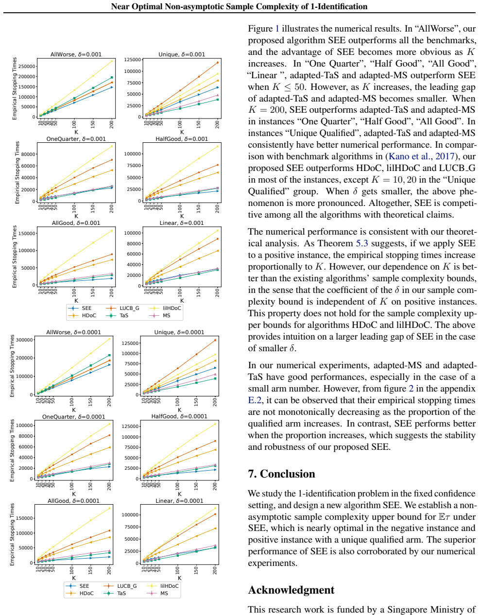
- Numerically, SEE's advantage over adapted-TaS and adapted-MS grows with $K$; if this persists, SEE is the more scalable choice for large screening problems, but the paper's experiments only cover Gaussian instances.
Editorial analysis
A structured set of objections, weighed in public.
Referee Report
Summary. The paper studies fixed-confidence 1-identification, where the agent must return an arm with mean at least a known threshold μ0 or return None, with error probability at most δ. The authors propose a new algorithm, Sequential-Explore-Exploit (SEE), which alternates between an exploration oracle (a modified LUCB-G step) and an exploitation oracle that certifies a candidate arm at the required confidence. The main theoretical contribution is Theorem 5.3, which gives non-asymptotic expected sample-complexity upper bounds of order γ(log(1/δ)/Δ²_{0,1} + log(K/Δ²_{0,1})·H^pos_1) for positive instances and γ·H^neg_1(log(1/δ)+log H^neg_1) for negative instances, together with a δ-PAC guarantee (Theorem 5.2). The paper then states lower bounds from prior work: Ω(H^neg_1 log(1/δ)) for negative instances (Theorem 5.4), Ω(log(1/δ)/Δ²_{0,1}) for positive instances (Theorem 5.5), and Ω(H_1) for a permuted positive instance under the extra condition μ1 > μ0 ≥ μ2 ≥ ⋯ ≥ μK (Theorem 5.6). The authors claim that the gap between these upper and lower bounds is at most a polynomial logarithmic factor, and support the algorithm with numerical experiments.
Significance. If the claims are correctly scoped, this is a useful step toward non-asymptotic algorithms for 1-identification. The negative case is well supported: the upper bound matches the lower bound up to a polylog H^neg_1 factor, and the δ-dependence of the positive-case upper bound matches the lower bound for all positive instances. The algorithm has no fitted parameters in the theory (only universal choices such as C = 1.01 and δ_k = 1/3^k), and the appendix provides a detailed proof structure with concentration and stopping-time arguments. The paper is also honest in places: it explicitly states in Section 5.2 that the tight δ-independent term is unclear when multiple arms exceed μ0, and the numerical section reports failure cases of APGAI. However, the advertised 'near optimality' in the abstract and Table 1 is broader than what the theorems establish, because the positive-case δ-independent lower bound is proven only for the unique-qualified-arm subcase, and even there only over a permutation. The contribution is therefore solid in the negative and unique-qualified positive regimes, but the general positive case remains open.
major comments (2)
- [Abstract; Table 1; Section 5.2] The abstract's claim of 'matching upper and lower bounds' and Table 1's '√' for the positive case are not supported for instances with two or more qualified arms. Theorem 5.3 gives an upper bound for every ν ∈ S_pos of γ(log(1/δ)/Δ²_{0,1} + log(K/Δ²_{0,1})·H^pos_1), but the only δ-independent lower bound for a positive instance, Theorem 5.6, is stated under the hypothesis μ1 > μ0 ≥ μ2 ≥ ⋯ ≥ μK, i.e., exactly one qualified arm. The paper itself concedes in Section 5.2 that the tight δ-independent term 'remains unclear' when there are multiple arms above μ0. Consequently, the near-optimality claim is proven only for the unique-qualified subcase, not for the general positive case, and the abstract/table should either be restricted accordingly or a matching lower bound for multi-qualified positive instances should be supplied.
- [Theorems 5.5 and 5.6 and the following discussion] The positive-case lower bound is existential over permutations rather than instance-wise. Theorem 5.6 guarantees that for any δ-PAC algorithm there exists a permutation ν of the given mean vector for which Eντ ≥ Ω(H1); it does not prove this bound for every permutation with those means. Since Theorem 5.3 gives an upper bound valid for every ν, the resulting gap comparison after Theorem 5.6 is a minimax statement over the class of permutations, not a per-instance near-optimality guarantee. The discussion should state this explicitly, or, if per-instance optimality is intended, provide an instance-wise lower bound.
minor comments (3)
- [Algorithm 2 and Appendix E.1] The default schedule in Algorithm 2 sets β_k = 2^k, while Appendix E.1 says the experiments use β_k = 2^k/4; this inconsistency should be reconciled, especially since the proof of Theorem 5.3 repeatedly uses β_k = 2^k.
- [Algorithm 5] In line 4 of Algorithm 5, the input arm is lowercase a but the sampling instruction reads 'Sample X ∼ νA'; the capital letter is a typographical distraction that should be fixed.
- [Table 1] The annotation in Table 1 for SEE, 'Even the O(log 1/Δ0,1) matches lower bound in some cases', is vague; the text should specify when this happens, e.g., in the small-Δ0,1 regime of Theorem 5.7, and what 'some cases' means.
Circularity Check
No circularity: the upper bound is proved from concentration and stopping-time arguments, the lower bounds are imported from independent prior work, and the acknowledged gap for multiple qualified arms is a scope limitation, not a circular reduction.
full rationale
The derivation chain is self-contained and non-circular. SEE's upper bound (Theorem 5.3) is obtained from concentration inequalities (Lemma D.3, adapted from Jamieson et al. 2014), stopping-time decompositions tau = tau_ee + tau_et, and probabilistic bounds on kappa_ee and kappa_et (Lemma 5.1), with no fitted parameters: C, delta_k, alpha_k, and beta_k are fixed universal schedules (Section 4.2). The lower bounds are quoted and adapted from independent prior work: Theorem 5.4 from Garivier & Kaufmann (2016) and Degenne & Koolen (2019); Theorem 5.5 from Kaufmann et al. (2016); Theorem 5.6 from Katz-Samuels & Jamieson (2020). None of these citations is a self-citation, and the lower-bound arguments do not presuppose SEE's stopping rule; they apply to any delta-PAC algorithm. The paper itself explicitly flags the one genuine limitation: Section 5.2 states that for instances with multiple arms above mu_0, 'it still remains unclear what would be a tight upper and lower bound of the delta independent part'. The abstract's unqualified 'near optimality' wording is broader than the theorem statements support, but that is a scope or overclaim issue, not a circular reduction of a prediction to its inputs. No quantity is fitted to data, no definition implicitly contains the target result, and no load-bearing conclusion is justified only by the authors' own prior work. Hence score 0.
Assumptions & free parameters
free parameters (4)
- C =
1.01
- δ_k =
1/3^k
- α_k =
5^k
- β_k =
2^k
assumptions (6)
- domain assumption Reward noises R_a - µ_a are 1-sub-Gaussian for all arms
- domain assumption The underlying instance is in S_pos ∪ S_neg, i.e., µ1 ≠ µ0
- domain assumption Arms can be relabeled so µ1 ≥ µ2 ≥ ... ≥ µK
- standard math Known external lower-bound theorems (Garivier and Kaufmann 2016; Degenne and Koolen 2019; Katz-Samuels and Jamieson 2020) apply to this setting
- standard math Lemma D.3 (union-bound concentration) holds uniformly over all times t
- standard math The stopping time τ is a stopping time with respect to the natural filtration
Cite this review
Pith. "Pith review of Near Optimal Non-asymptotic Sample Complexity of 1-Identification." pith.science (2026). https://pith.science/paper/5Q245JXN
@misc{pith2026250606978,
  author       = {Pith},
  title        = {Pith review of: Near Optimal Non-asymptotic Sample Complexity of 1-Identification},
  year         = {2026},
  howpublished = {\url{https://pith.science/paper/5Q245JXN}},
  note         = {Machine review of arXiv:2506.06978}
}
abstract
Motivated by an open direction in existing literature, we study the 1-identification problem, a fundamental multi-armed bandit formulation on pure exploration. The goal is to determine whether there exists an arm whose mean reward is at least a known threshold $\mu_0$, or to output None if it believes such an arm does not exist. The agent needs to guarantee its output is correct with probability at least $1-\delta$. Degenne & Koolen 2019 has established the asymptotically tight sample complexity for the 1-identification problem, but they commented that the non-asymptotic analysis remains unclear. We design a new algorithm Sequential-Exploration-Exploitation (SEE), and conduct theoretical analysis from the non-asymptotic perspective. Novel to the literature, we achieve near optimality, in the sense of matching upper and lower bounds on the pulling complexity. The gap between the upper and lower bounds is up to a polynomial logarithmic factor. The numerical result also indicates the effectiveness of our algorithm, compared to existing benchmarks.
Figures

Reference graph
Works this paper leans on
-
[1]
Na(Hee) ≤ max ( N 0 a , 113(C+1)2(log 2K δ +log log 96(C+1)2 max{∆2 0,a ,∆2 1,a } ) max{∆2 0,a,∆2 1,a} ) , for a ∈ [K]
-
[2]
ˆa ∈ [K], µˆa > ωµ1 + (1 − ω)µ0, ω = C−1 C+3 . Proof of Lemma B.4. For simplicity, denote T ′ a = 113(C+1)2(log 2K δ +log log 96(C+1)2 ∆2 1,a ) ∆2 1,a , T ′′ a = 113(C+1)2(log 2K δ +log log 96(C+1)2 ∆2 0,a ) ∆2 0,a . Not hard to see min{T ′ a , T ′′ a } = 113(C+1)2(log 2K δ +log log 96(C+1)2 max{∆2 0,a ,∆2 1,a } ) max{∆2 0,a,∆2 1,a} . Consider a ≥ 2. For ...
-
[3]
The term 1 ϵ2 implies the upper bound can be infinity. And the term H1 log log(1/δ) suggests there is still gap between the upper and lower bounds. Regarding algorithm APGAI, (Jourdan & R´eda, 2023) do not explicitly provide upper bound forEτ. Therorem 2 in (Jourdan & R´eda, 2023) suggests Eντ ≤ Cpos(δ) + Kπ 2 6 + 1, ν∈ Spos Eντ ≤ Cneg(δ) + Kπ 2 6 + 1, ν∈...
work page 2023
-
[7]
If N 0 a ≤ T′ a ≤ T′′ a , the algorithm assures Na(Hee) ≤ T′ a = max ( N 0 a , 113(C+1)2(log 2K δ +log log 96(C+1)2 max{∆2 0,a ,∆2 1,a } ) max{∆2 0,a,∆2 1,a} ) , as UCBa < µ1 < UCB1 ⇐ Na(Hee) ≥ 112 log 2K δ ∆2 1,a + 64 log log 96 ∆2 1,a ∆2 1,a + 1and arm a will never be the arm with highest upper confidence bound before Na(Hee) is no less than T ′ a
-
[8]
If T ′ a < N0 a ≤ T′′ a , the algorithm never pulls arm a as its upper bound must below arm 1. In this case, Na(Hee) ≤ N 0 a = max ( N 0 a , 113(C+1)2(log 2K δ +log log 96(C+1)2 max{∆2 0,a ,∆2 1,a } ) max{∆2 0,a,∆2 1,a} )
-
[9]
If If N 0 a ≤ T′′ a ≤ T′ a, the algorithm assures Na(Hee) ≤ T′′ a = max ( N 0 a , 113(C+1)2(log 2K δ +log log 96(C+1)2 max{∆2 0,a ,∆2 1,a } ) max{∆2 0,a,∆2 1,a} ) , as the algorithm will output arm a before its pulling time is no less than T ′′ a . By the first claim, we know KX a=1 Na(Hee) ≤ KX a=1 max N 0 a , 113(C + 1)2(log 2K δ + log log 96(C+1)2...
-
[10]
Na(Hee) ≤ max ( N 0 a , 113(log 2K δ +log log 96 ∆2 0,a ) ∆2 0,a ) , for ∀a ∈ [K]
-
[11]
For simplicity, denote Ta = 113(log 2K δ +log log 96 ∆2 0,a ) ∆2 0,a
ˆa ∈ None Proof of Lemma B.5. For simplicity, denote Ta = 113(log 2K δ +log log 96 ∆2 0,a ) ∆2 0,a . Consider a ≥ 1. For pulling times t ∈ N, through the following calculation, Pt s=1 Xee a,s t + U (t, δ K ) < µ0 Eee ⇐µa + 2 · U (t, δ K ) < µ0 ⇐2 s 4 log 2K log(2t) δ t ≤ ∆0,a Lemma D.2 ⇐ t > 112(log 2K δ + log log 96 ∆2 0,a ) ∆2 0,a , we know UCBa(t) < µ0...
Show all 13 references
-
[12]
23 Near Optimal Non-asymptotic Sample Complexity of 1-Identification
If N 0 a ≤ Ta, the algorithm assures Na(Hee) ≤ Ta = max{N 0 a , Ta}, as the above discussion indicates. 23 Near Optimal Non-asymptotic Sample Complexity of 1-Identification
-
[13]
AllWorse
If N 0 a > Ta, then the upper confidence bound of arm a is smaller than the µ0 at the start of the algorithm. This arm will never get pull till the end of the algorithm. Thus, Na(Hee) = N 0 a = max{N 0 a , Ta}. Then, we turn to the second claim. From the good event, we know LC...
2016
-
[1791]
Kaufmann, E
PMLR, 2020. Kaufmann, E. and Kalyanakrishnan, S. Information com- plexity in bandit subset selection. InConference on Learn- ing Theory, pp. 228–251. PMLR, 2013. Kaufmann, E., Capp ´e, O., and Garivier, A. On the com- plexity of best arm identification in multi-armed bandit mo...
2020 arXiv
-
[2017]
aim to output all the arm sequentially and its first outputting round is indeed the τ. Besides the fixed confidence setting adopted by the above papers, (Locatelli et al., 2016; Mukherjee et al., 2017) work on the fixed budget setting, which aims to maximize the probability of...
2016
-
[2020]
The sub-optimality of the above upper bound mainly comes from two parts
coupled with the stopping time λ1. The sub-optimality of the above upper bound mainly comes from two parts. Firstly, the dependence on δ is log 1 δ log log 1 δ instead of the commonly seen result log 1 δ . Then, in the asymptotic regime, i.e. δ → 0, this upper bound is larger ...
2020
Reviewed August 7, 2026 · model on record in the stance chip above.
Discussion (0). Sign in to comment.