REVIEW 4 major objections 6 minor 35 references
New highly efficient and accurate numerical scheme for the Cahn-Hilliard-Brinkman system
T0 review · 4 major / 6 minor · reviewed 2026-08-07 · deepseek-v4-flash
Pith's one-line read A variable-time-step BDF-SAV scheme is proved unconditionally energy-stable for the Cahn-Hilliard-Brinkman system.
desk verdict Variable-step BDFk R-GSAV for Cahn-Hilliard-Brinkman is a useful, mostly sound contribution, but the manuscript under-specifies the chemical-potential update and has coefficient typos that a revision should fix. read the letter →
The pith
A machine-rendered reading of the paper's core claim, the machinery that carries it, and where it could break.
The reading
What carries the argument
The load-bearing object is the relaxed generalized scalar auxiliary variable $r(t)=E_1(\varphi(t))$ together with the relaxation correction in (2.4g) and (2.5). The proof mechanism is the case analysis of Theorem 2.1: choosing $\sigma^{n+1}_0$ and $\delta^{n+1}$ according to whether the intermediate value $\tilde{r}^{n+1}$ is above, below, or equal to $E_1(\varphi^{n+1})$ makes the discrete energy identity $r^{n+1} - r^n = -\tau_{n+1}\delta^{n+1}\kappa(\varphi^{n+1},u^{n+1})$ hold, where $\kappa(\varphi,u)$ is the integral of the dissipative terms from the continuous energy law. This identity is what enforces both unconditional energy decay and the bound $r^{n+1} \le E_1(\varphi^{n+1})$, keeping the modified energy close to the physical free energy.
What would settle it
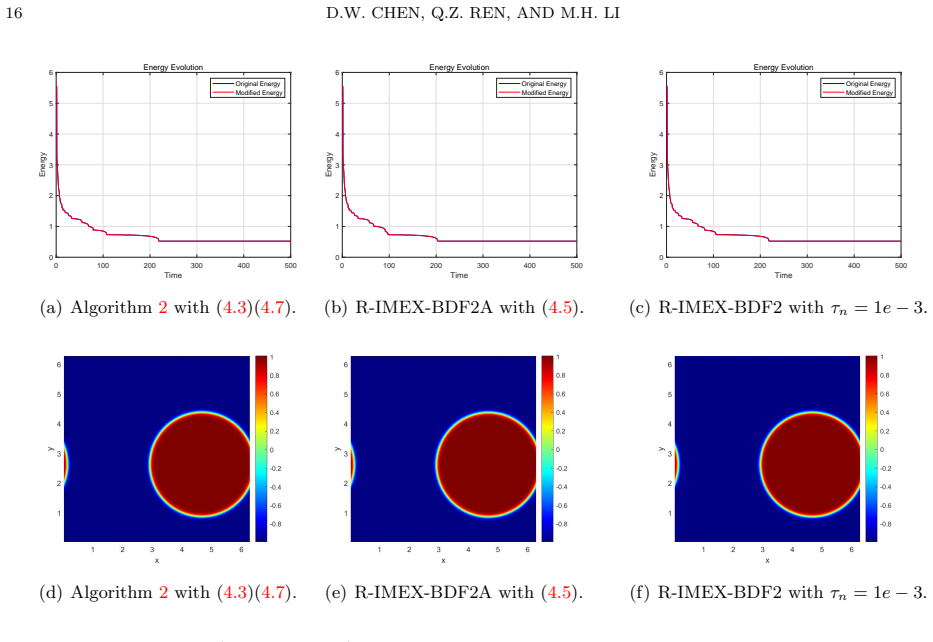
Run Scheme 1 on the Example 4.3 coarsening benchmark with time-step ratios above 4.8645, as produced by Algorithm 2 in Figure 4.6, and monitor $r^{n+1}-r^n$: any positive value would contradict Theorem 2.1; alternatively, benchmark Algorithm 2 against fixed-step R-IMEX-BDF2 at matched $L^2$ error and CPU time on a parameter set outside (4.3)-(4.8), where a cheaper fixed-step run would refute the reported efficiency advantage.
Extended reading notes
Core claim
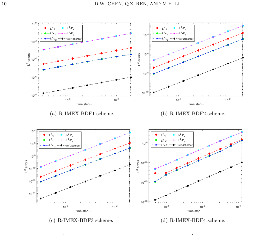
The core claim is that the CHB system can be solved by R-IMEX-BDFk schemes, $k=1,2,3,4$, that combine an implicit-explicit BDF discretization with a relaxed scalar auxiliary variable. The auxiliary variable is defined as $r(t)=E_1(\varphi)=E(\varphi)+C_0$, and the scheme first computes an intermediate phase field, velocity, pressure, and auxiliary value, then corrects with a relaxation factor $\zeta^{n+1}_k = 1 - (1-\xi^{n+1}_k)^{k+1}$. Theorem 2.1 specifies four cases for choosing the relaxation parameter $\sigma^{n+1}_0$ and the nonnegative dissipation parameter $\delta^{n+1}$ so that $r^{n+1}$ is both nonincreasing and bounded above by the physical energy $E_1(\varphi^{n+1})$. This transfers the continuous dissipation law to the discrete level without restricting the ratio of adjacent time steps, which is the property that makes the subsequent adaptive algorithms possible.
Load-bearing premise
The adaptive efficiency claims rest on the untested assumption that $|1-\xi^{n+1}_k|^m$, with a manually chosen exponent $m$ in $(0,1)$, is a reliable proxy for the numerical error of the coupled CHB solution, and on a hand-picked switching time $T_c$; the paper offers no error analysis for either, and its own Table 4.4 shows that R-IMEX-BDF2A alone gives meaningless results for parameter sets (4.7) and (4.8).
Editorial extensions
If this is right
- For any sequence of time steps, including ratios far above the previously noted bound 4.8645, the modified energy $r^n$ never increases, so no CFL-type step restriction is needed for stability.
- The relaxation improves accuracy over plain IMEX-BDF at large time steps, as shown in Table 4.1, where the unrelaxed second-order scheme develops large errors at $\tau=2\times10^{-3}$ while the relaxed scheme remains accurate.
- The hybrid-order Algorithm 2, using R-IMEX-BDF3A on $[0,T_c]$ and R-IMEX-BDF2A on $(T_c,T]$, is reported to cut CPU time by factors of roughly two to four against fixed-step R-IMEX-BDF2 at similar error and to beat IMEX-CNA in both accuracy and cost.
- The same R-GSAV construction is claimed to extend directly to other phase-field equations, since the relaxation and adaptive error indicator do not rely on CHB-specific structure beyond the energy law.
- The adaptive algorithms inherit the unconditional energy stability of the base scheme, so the modified energy remains monotone even when the step-size ratio fluctuates, as demonstrated in Figures 4.6 and 4.7.
Reading between the lines
- The error indicator $|1-\xi^{n+1}_k|^m$, with a manually chosen exponent $m\in(0,1)$, is empirical rather than derived; a rigorous a posteriori bound linking it to the actual phase-field error would put the adaptive algorithms on the same footing as the stability theorem.
- The switch time $T_c$ is hand-picked by observing where the fast transient ends; an automatic rule based on when $E'(t)$ or the step-size history crosses a threshold could make the hybrid algorithm self-tuning and more robust across different problems.
- The stability proof guarantees decay of the modified energy $r^{n+1}$ but does not quantify the gap between $r^{n+1}$ and the original free energy $E(\varphi^{n+1})$; a step-size-dependent bound on that gap would tell users how much the modified energy can be trusted as a physical diagnostic.
- Because the construction only uses the energy-dissipation structure, the hybrid-order adaptive strategy is a plausible candidate for other coupled phase-field systems, such as phase-field crystal or tumor-growth models, where high-order BDF schemes suffer the same early-transient versus long-time stability trade-off.
Editorial analysis
A structured set of objections, weighed in public.
Referee Report
Summary. The paper proposes a class of variable-time-step backward differentiation formula (BDF) schemes for the Cahn-Hilliard-Brinkman (CHB) system, built on a generalized scalar auxiliary variable (GSAV) approach with relaxation (R-GSAV). The schemes are claimed to be unconditionally energy-stable in a modified (SAV) energy, and the authors design adaptive time-stepping strategies, including a hybrid-order algorithm that switches between BDF3 and BDF2 according to a user-specified time Tc. Numerical experiments report temporal convergence rates for k=1,...,4, long-time coarsening simulations, and comparisons of CPU time and accuracy for the adaptive algorithms against fixed-step and existing adaptive schemes.
Significance. If substantiated, the paper would provide a useful extension of R-GSAV relaxation to the coupled CHB system, and the proposed hybrid adaptive strategy is a pragmatic idea for combining the short-time accuracy of BDF3 with the long-time robustness of BDF2. The central energy-decay identity r^{n+1}-r^n = -τ δ κ ≤ 0 is essentially algebraic and, under a consistent definition of the auxiliary variables, should hold for any nonnegative κ. However, the manuscript currently suffers from an under-specified scheme, coefficient typos, missing forcing terms in the accuracy test, and a strong dependence of the advertised adaptive gains on hand-tuned parameters. These issues prevent the main claims from being verified as written.
major comments (4)
- [Section 2.2, Scheme 1 (2.4a)-(2.4g)] The scheme does not specify how the chemical potential μ^{n+1} is updated. Step 1 defines an intermediate μ̃ and then (2.4g) rescales only φ, u, and p, leaving μ undefined. This is not a cosmetic omission: the next time step needs B_k(μ^n) in (2.4c), and Theorem 2.1's κ(φ^{n+1}, u^{n+1}) in (2.6)-(2.7) depends on μ^{n+1}. If μ^{n+1} is silently set to ζ μ̃, then κ(φ^{n+1}, u^{n+1}) is not the dissipation rate of the accepted state because M(ζφ̃)|∇(ζμ̃)|² ≠ ζ²M(φ̃)|∇μ̃|² for general mobility M; if μ^{n+1} is instead defined as the physical chemical potential -ε²Δφ^{n+1}+F'(φ^{n+1}), then μ^{n+1} ≠ ζ μ̃ because F' is cubic. The paper must state the update rule for μ and show that the relation between (2.4e) and (2.6) is meaningful under that rule; otherwise both the unconditional energy-stability theorem and the reported convergence rates rest on an unstated convention.
- [Section 2.2, coefficient formulas for A_k and B_k] The printed formulas for the second- and third-order coefficients contain sign and denominator errors. For k=2, A2(φ^n) is printed with a leading term (-t_{n+1}+t_{n-1})/(t_n-t_{n-1}) φ^n, which equals -(1+τ_{n+1}/τ_n)φ^n, together with a second term -τ_{n+1}²/(τ_n(τ_n+τ_{n+1}))φ^{n-1}; the standard nonuniform BDF2 coefficient A2 should be +(1+τ_{n+1}/τ_n)φ^n - τ_{n+1}²/(τ_n(τ_n+τ_{n+1}))φ^{n-1}. For k=3, B3(φ^n) contains denominators such as (t_n+t_{n-2}) and (t_{n-1}+t_{n-2}), which should be differences (t_n-t_{n-2}) and (t_{n-1}-t_{n-2}). As written, the R-IMEX-BDF2 and R-IMEX-BDF3 schemes are not the claimed high-order BDF discretizations and cannot be implemented. Corrected coefficient formulas for k=2,3,4 should be provided.
- [Section 4.1, Example 4.1] The accuracy test does not state that manufactured source terms are added to the CHB system. The exact solution (4.1) does not satisfy the homogeneous CHB equations (2.1) with the given parameters (ε=1, γ=2, M=ν=η=1, S=0); for instance, μ=φ³+φ and φ_t=-sin(t)cos(x)sin(y), so (2.1a) cannot hold without an external forcing term. The paper must specify the added forcing terms for the manufactured solution, or the convergence orders reported in Figure 4.1 cannot be reproduced.
- [Section 3 and Table 4.4] The robustness of the proposed adaptive algorithms is not established. The paper states in Section 3 that the error indicator |1-ξ_k|^m works when m is 'appropriately chosen between 0 and 1', but no selection rule or theory is given. Table 4.4 shows that R-IMEX-BDF2A with parameter sets (4.7) and (4.8) yields 'meaningless solutions', while Algorithm 2 succeeds under the same settings. Since the claimed efficiency of the hybrid algorithm depends on the hand-picked parameters (ρ, tol, r, m, τ_max) and the switch time Tc, the paper should provide a systematic parameter-selection strategy or at least a sensitivity study, and it should clarify why the hybrid algorithm is robust when the underlying single-order adaptive algorithms fail.
minor comments (6)
- [Section 2.1, equations (2.2a)-(2.3)] The derivation of the dissipation law appears to add (2.2b) to (2.2a) and (2.2c), although (2.2a) already contains (φ_t, μ); adding (2.2b) double-counts and would introduce a spurious factor 1/2. The correct step is to use (2.2b) to replace (φ_t, μ) with dE/dt. Please clarify the intended derivation.
- [Theorem 2.1 proof, equation (2.9)] The proof assumes E1(φ̃^{n+1}) ≥ 0 and then divides by E1 in (2.4e) and (2.9). With C0=0, E1 can be arbitrarily close to zero or exactly zero for constant states, making the division undefined. The theorem should assume E1(φ̃^{n+1}) > 0, or require C0 > 0, or discuss how zero-energy states are handled.
- [Remark 2.2, inequality (2.11)] The bound (Lφ^{n+1}, φ^{n+1}) ≤ (C_k M)^2 appears to require (Lφ̃, φ̃) ≤ E1(φ̃), but from the definition E1 = 1/2(Lφ̃, φ̃) + ∫F, only (Lφ̃, φ̃) ≤ 2E1(φ̃) holds under nonnegativity of F. The displayed square (Lφ̃, φ̃)^2 in (2.11) seems erroneous; please check the estimate.
- [Algorithms 1 and 2] The adaptive algorithms use E'(t) without defining its discrete counterpart; specify whether E'(t) is approximated by a finite difference of the discrete energy, and with which step size.
- [Algorithm 1, Step 4] In Step 4, the update formula Adp(e_n^{m_k}, τ_{n+1}) uses τ_{n+1} before τ_{n+1} has been computed; this should presumably be Adp(e_n^{m_k}, τ_n) or a clearly defined preliminary value.
- [Algorithm 2, Steps 1 and 6] The notation 'compute ξ_n by the R-IMEX-BDF3/BDF2' is inconsistent with the earlier definition ξ_k^{n+1}; this should be ξ^{n+1}_3 and ξ^{n+1}_2 respectively.
Circularity Check
The energy-stability theorem is self-definitional: the relaxation set Γ in (2.6) is defined by the very decay identity that Theorem 2.1 then 'proves', so the central stability claim reduces to a construction rather than an independent derivation.
-
self definitional
[Section 2.2, equations (2.5)-(2.7) and Theorem 2.1]
"Step2:Compute scalar auxiliary variable rn+1 by using the following relaxation: rn+1 = σn+1 0 ˜rn+1 + (1 − σn+1 0 )E1(ϕn+1), σn+1 0 ∈ Γ, (2.5) where Γ = { σ ∈ [0, 1] s.t. rn+1 − ˜rn+1 / τn+1 = −δn+1κ(ϕn+1, un+1) + ˜rn+1 / E1( ˜ϕn+1) κ( ˜ϕn+1, ˜un+1) }, (2.6) with δn+1 ⩾ 0 to be determined. The following theorem summarizes the selection of σn+1 0 and δn+1. ... Given rn ⩾ 0, we have rn+1 ⩾ 0, ξn+1 k ⩾ 0 in the scheme (2.4)-(2.5) and rn+1 is unconditionally energy stable in the sense that rn+1 − rn = −τn+1δn+1κ(ϕn+1, un+1) ≤ 0"
Equation (2.6) defines Γ as the set of relaxation parameters for which the target decay equality holds after combining with (2.4e). Theorem 2.1 then chooses σ0 and δ from that set and derives (2.7) by combining (2.4e) with (2.6). Thus the unconditional energy-stability inequality is not a consequence of the discretized CHB equations; it is the defining constraint of the relaxation step. The case analysis only checks that the proposed σ0,δ satisfy σ0∈[0,1], δ≥0, and r≤E1; the decay statement itself is a restatement of the definition of Γ. This is the standard SAV construction, but as a 'strict proof' of energy stability it is self-definitional.
full rationale
The central advertised result (Theorem 2.1) is a construction: the relaxation step (2.5)-(2.6) defines Γ by the very decay equality that the theorem asserts, so the proof that r^{n+1}-r^n = -τδκ ≤ 0 is an algebraic consequence of the definition of δ, not an independent derivation. This is a genuine self-definitional element in the main stability claim. I nevertheless keep the score at 6 rather than higher because the numerical content of the paper is not entirely circular: convergence rates in Example 4.1 are measured against the manufactured exact solution (4.1), and the adaptive/coarsening tests use an independent τ=1e-6 reference solution, so accuracy claims are externally benchmarked. The adaptive error indicator |1-ξ|^m and the switch time Tc are empirical/heuristic (Section 3), with the paper itself reporting failures for parameter sets (4.7)-(4.8) in Table 4.4; this is tuning, not a fitted parameter renamed as a prediction, so it does not add circularity. I find no load-bearing self-citation chain: the underlying SAV/relaxation framework is credited to [33] and [35], which are not invoked as an unverified uniqueness theorem, and the stability proof does not depend on the authors' own prior results. Separately, the scheme as written never updates μ^{n+1}: Step 1 defines φ̃, μ̃, ũ, p̃, r̃ and then rescales φ,u,p but not μ, while (2.4c) and κ(φ^{n+1},u^{n+1}) require μ; this is a formal well-definedness gap in Theorem 2.1 and the algorithm, but it is a correctness issue rather than a circularity and is not scored.
Assumptions & free parameters
free parameters (5)
- S (stabilization parameter) =
S=0 (Example 4.1), S=1 (Examples 4.2-4.4)
- C0 (energy shift) =
C0=0
- m (error indicator exponent) =
0.52, 0.70, 0.75, 0.85, 0.68, 0.70 in (4.3)-(4.8); m=1 in (4.9)-(4.10)
- Adaptive controller parameters rho, tol, r, gamma*, tau_min, tau_max =
six sets (4.3)-(4.8) and (4.9)-(4.10)
- Tc (switch time) =
Tc=1.2 in Example 4.3; Tc=0.4 in Example 4.4
assumptions (4)
- domain assumption The continuous CHB system (2.1) has solutions and satisfies the energy law (2.3) for the data considered.
- ad hoc to paper E1(phi~^{n+1}) > 0 at every step wherever the scheme divides by it in (2.4e), (2.4f), (2.9)-(2.11).
- ad hoc to paper |1-xi|^m is a reliable error indicator for the CHB system for suitably chosen m.
- domain assumption The standard BDF variable-step coefficient formulas from [20] produce kth-order accuracy.
Cite this review
Pith. "Pith review of New highly efficient and accurate numerical scheme for the Cahn-Hilliard-Brinkman system." pith.science (2026). https://pith.science/paper/DPCYUN6U
@misc{pith2026250607128,
  author       = {Pith},
  title        = {Pith review of: New highly efficient and accurate numerical scheme for the Cahn-Hilliard-Brinkman system},
  year         = {2026},
  howpublished = {\url{https://pith.science/paper/DPCYUN6U}},
  note         = {Machine review of arXiv:2506.07128}
}
read the original abstract
In this paper, based on a generalized scalar auxiliary variable approach with relaxation (R-GSAV), we construct a class of high-order backward differentiation formula (BDF) schemes with variable time steps for the Cahn-Hilliard-Brinkman(CHB) system. In theory, it is strictly proved that the designed schemes are unconditionally energy-stable. With the delicate treatment of adaptive strategies, we propose several adaptive time-step algorithms to enhance the robustness of the schemes. More importantly, a novel hybrid-order adaptive time steps algorithm performs outstanding for the coupled system. The hybrid-order algorithm inherits the advantages of some traditional high-order BDF adaptive strategies. A comprehensive comparison with some adaptive time-step algorithms is given, and the advantages of the new adaptive time-step algorithms are emphasized. Finally, the effectiveness and accuracy of the new methods are validated through a series of numerical experiments.
Figures


Figures from the paper (6 more)



Reference graph
Works this paper leans on
-
[35]
N. Zheng and X. Li, New efficient and unconditionally energy stable schemes for the cahn– hilliard–brinkman system , Appl. Math. Lett., 128 (2022), p. 107918
work page 2022
-
[21]
P. Jiang, H. Jia, L. Liu, C. Zhang, and D. W ang, Highly efficient, robust and uncon- ditionally energy stable second order schemes for approximating the cahn-hilliard-brinkman system, Appl. Numer. Math., 201 (2024), pp. 175–186. NEW SCHEMES FOR THE CAHN-HILLIARD-BRINKMAN SYSTEM 21
work page 2024
-
[1]
D. M. Anderson, G. B. McF adden, and A. A. Wheeler, Diffuse-interface methods in fluid mechanics, Annu. Rev. Fluid Mech., 30 (1998), pp. 139–165
work page 1998
-
[2]
L. Chen and C. Xu, A time splitting space spectral element method for the cahn-hilliard equation, East Asian J. Appl. Math., 3 (2013), pp. 333–351
work page 2013
-
[3]
L. Chen and J. Zhao, A novel second-order linear scheme for the cahn-hilliard-navier-stokes equations, J. Comput. Phys., 423 (2020), p. 109782
work page 2020
-
[4]
Y. Chen, Y. Huang, N. Yi, and P. Yin, Recovery type a posteriori error estimation of an adaptive finite element method for cahn–hilliard equation , J. Sci. Comput., 98 (2024), p. 35. 20 D.W. CHEN, Q.Z. REN, AND M.H. LI
work page 2024
-
[5]
Q. Cheng and J. Shen, Multiple scalar auxiliary variable (MSA V) approach and its applica- tion to the phase-field vesicle membrane model , SIAM J. Sci. Comput., 40 (2018), pp. A3982– A4006
work page 2018
- [6]
Show all 35 references
-
[7]
Collins, J
C. Collins, J. Shen, and S. M. Wise, An efficient, energy stable scheme for the cahn- hilliard-brinkman system , Commun. Comput. Phys., 13 (2013), pp. 929–957
2013
-
[8]
Conti and A
M. Conti and A. Giorgini, Well-posedness for the brinkman–cahn–hilliard system with unmatched viscosities, J. Differ. Equ., 268 (2020), pp. 6350–6384
2020
-
[9]
Ebenbeck and H
M. Ebenbeck and H. Garcke, On a cahn–hilliard–brinkman model for tumor growth and its singular limits , SIAM J. Math. Anal., 51 (2019), pp. 1868–1912
2019
-
[10]
Ebenbeck, H
M. Ebenbeck, H. Garcke, and R. N¨urnberg, Cahn–hilliard–brinkman systems for tumour growth, Discrete Contin. Dyn. Syst. - S., 14 (2021), pp. 3989–4033
2021
-
[11]
Feng and H
X. Feng and H. Wu, A posteriori error estimates for finite element approximations of the cahn-hilliard equation and the hele-shaw flow , J. Comput. Math., (2008), pp. 767–796
2008
-
[12]
U. S. Fjordholm, S. Mishra, and E. Tadmor, Well-balanced and energy stable schemes for the shallow water equations with discontinuous topography , J. Comput. Phys., 230 (2011), pp. 5587–5609
2011
-
[13]
Garcke, K
H. Garcke, K. F. Lam, E. Sitka, and V. Styles, A cahn–hilliard–darcy model for tumour growth with chemotaxis and active transport , Math. Models Methods Appl. Sci., (2016)
2016
-
[14]
R. Guo, Y. Xia, and Y. Xu, An efficient fully-discrete local discontinuous galerkin method for the cahn–hilliard–hele–shaw system , J. Comput. Phys., 264 (2014), pp. 23–40
2014
-
[15]
Han and X
D. Han and X. W ang, A second order in time, uniquely solvable, unconditionally stable numerical scheme for cahn–hilliard–navier–stokes equation , J. Comput. Phys., 290 (2015), pp. 139–156
2015
-
[16]
, A second order in time, decoupled, unconditionally stable numerical scheme for the cahn– hilliard–darcy system, J. Sci. Comput., 77 (2018), pp. 1210–1233
2018
-
[17]
Hou and Z
D. Hou and Z. Qiao, An implicit–explicit second-order bdf numerical scheme with variable steps for gradient flows , J. Sci. Comput., 94 (2023), p. 39
2023
-
[18]
Methods Partial Differ
, A linear adaptive second-order backward differentiation formulation scheme for the phase field crystal equation , Numer. Methods Partial Differ. Equ., 39 (2023), pp. 4174–4195
2023
-
[19]
Huang and J
F. Huang and J. Shen, A new class of implicit–explicit bdfk sav schemes for general dissipa- tive systems and their error analysis , Comput. Meth. Appl. Mech. Eng., 392 (2022), p. 114718
2022
-
[20]
Huang, J
F. Huang, J. Shen, and Z. Yang, A highly efficient and accurate new scalar auxiliary variable approach for gradient flows , SIAM J. Sci. Comput., 42 (2020), pp. A2514–A2536
2020
-
[22]
Knopf and A
P. Knopf and A. Signori, Existence of weak solutions to multiphase cahn–hilliard–darcy and cahn–hilliard–brinkman models for stratified tumor growth with chemotaxis and general source terms, Commun. Partial Differ. Equ., 47 (2022), pp. 233–278
2022
-
[23]
Le Bars and M
M. Le Bars and M. G. Worster, Interfacial conditions between a pure fluid and a porous medium: implications for binary alloy solidification , J. Fluid Mech., 550 (2006), pp. 149–173
2006
-
[24]
Li and C
M. Li and C. Xu, New efficient time-stepping schemes for the navier–stokes–cahn–hilliard equations, Comput. Fluids., 231 (2021), p. 105174
2021
-
[25]
Li and J
X. Li and J. Shen, On a sav-mac scheme for the cahn–hilliard–navier–stokes phase-field model and its error analysis for the corresponding cahn–hilliard–stokes case , Math. Models Methods Appl. Sci., 30 (2020), pp. 2263–2297
2020
-
[26]
H.-l. Liao, B. Ji, and L. Zhang, An adaptive bdf2 implicit time-stepping method for the phase field crystal model , IMA J. Numer. Anal., 42 (2022), pp. 649–679
2022
-
[27]
C. Liu, J. Shen, and X. Yang, Decoupled energy stable schemes for a phase-field model of two-phase incompressible flows with variable density , J. Sci. Comput., 62 (2015), pp. 601–622
2015
-
[28]
Ngamsaad, J
W. Ngamsaad, J. Yojina, and W. Triampo, Theoretical studies of phase-separation ki- netics in a brinkman porous medium , J. Phys. A-Math. Theor., 43 (2010), p. 202001
2010
-
[29]
J. Shen, J. Xu, and J. Yang, The scalar auxiliary variable (SA V) approach for gradient flows, J. Comput. Phys., 353 (2018), pp. 407–416
2018
-
[30]
Shen and X
J. Shen and X. Yang, Numerical approximations of Allen-Cahn and Cahn-Hilliard equations, Discrete Contin. Dyn. Syst., 28 (2010), pp. 1669–1691
2010
-
[31]
W ang and S
C. W ang and S. M. Wise, An energy stable and convergent finite-difference scheme for the modified phase field crystal equation , SIAM J. Numer. Anal., 49 (2011), pp. 945–969
2011
-
[32]
N. K. Yamaleev and M. H. Carpenter, A systematic methodology for constructing high- order energy stable weno schemes , J. Comput. Phys., 228 (2009), pp. 4248–4272
2009
-
[33]
Zhang and J
Y. Zhang and J. Shen, A generalized sav approach with relaxation for dissipative systems , J. Comput. Phys., 464 (2022), p. 111311
2022
-
[34]
Zhang, Y
Z. Zhang, Y. Ma, and Z. Qiao, An adaptive time-stepping strategy for solving the phase field crystal model , J. Comput. Phys., 249 (2013), pp. 204–215
2013
Reviewed August 7, 2026 · model on record in the stance chip above.
Discussion (0). Sign in to comment.