REVIEW 3 major objections 6 minor 26 references
Improving Memory Efficiency for Training KANs via Meta Learning
T0 review · 3 major / 6 minor · reviewed 2026-08-07 · deepseek-v4-flash
Pith's one-line read KANs' trainable parameters can be cut to roughly MLP level by replacing direct weight optimization with a small meta-learner that generates every spline coefficient from a per-connection scalar prompt, while the paper reports matching or…
desk verdict A real hypernetwork-for-KANs idea with broad experiments, but the scalar-prompt formulation in Eq. (9) is not what the best results use, making the headline parameter reduction overstated. read the letter →
The pith
A machine-rendered reading of the paper's core claim, the machinery that carries it, and where it could break.
The reading
What carries the argument
The load-bearing object is the weight-generation map $M_\theta(z)=w$, a two-layer MLP with hidden dimension $d_{\mathrm{hidden}}$ that takes the scalar prompt of one activation and outputs its $G+k+1$ spline coefficients. The prompt $z$ is the learned identifier of the univariate function, the meta-learner is the shared rule for translating identifiers into coefficients, and the activation becomes $\phi(t; z,\theta)=M_\theta(z)^\top B(t)$. For deep KANs the machinery adds a clustering step that groups layers by their channel sizes and assigns each cluster a separate $M_\theta^{(c)}$, trading a small constant parameter overhead for the ability to learn layer-dependent rules.
What would settle it
Train a MetaKAN and a direct KAN on a target where two edges in the same layer must represent sharply different univariate functions, such as one highly oscillatory edge and one nearly constant edge, using the same optimization budget. If the shared meta-learner with scalar prompts cannot match the direct KAN's accuracy at any hidden width, the scalar-prompt assumption fails.
Extended reading notes
Core claim
The paper's central claim is that the univariate functions inside a KAN are not independent tasks: they all belong to a shared functional class $\mathcal{F} = \{f \mid f(t)=w^\top B(t), w\in\mathbb{R}^{G+k+1}\}$, so the rule that maps a function's identity to its spline coefficients can be learned once and reused. MetaKANs implement that rule as $M_\theta: \mathbb{R}\to\mathbb{R}^{G+k+1}$, with a learnable scalar prompt $z$ for each activation standing in for the function's identity. Training proceeds end-to-end on the original loss, updating both prompts and meta-learner. For deep KANs, layers with similar channel dimensions are clustered by width and each cluster receives its own meta-learner, keeping cost under control. The claimed outcome is that the generated weights match or beat directly optimized KAN weights while the trainable parameter count drops to approximately that of an MLP.
Load-bearing premise
A single scalar prompt per activation carries enough information to identify the correct univariate function, so one shared meta-learner can generate near-optimal coefficients for every edge.
Editorial extensions
If this is right
- Peak memory during training falls to near-MLP levels, with the largest savings reported at large grid sizes such as $G=80$ and above.
- The meta-learner recipe is model-agnostic: applying it to FastKAN, WavKAN, and ConvKAN cuts their parameter counts by roughly $1/\dim(w)$ while keeping competitive accuracy.
- Deep KANs become more scalable, because the meta-learner cost $C(d_{\mathrm{hidden}}+1)(G+k+1)$ stays small and fixed while the prompt count grows only with the number of connections.
- For very small KANs the fixed meta-learner cost can exceed the spline parameters it replaces, so MetaKANs can have slightly more parameters than KANs in that regime even when accuracy stays competitive.
Reading between the lines
- If scalar prompts truly identify the needed univariate functions, then prompt geometry is a compact summary of what the network learned; a natural test is whether interpolation or clustering of prompts transfers between tasks or architectures.
- The meta-learner imposes a strong shared-structure prior, which may explain the accuracy gains and improved compactness; a direct check is whether MetaKANs beat KANs on out-of-distribution inputs, not just on the training distribution.
- The layer-clustering rule suggests that the number of meta-learners should track the diversity of layer widths rather than depth itself, so adding layers within a width cluster could add almost no parameters.
- A concrete extension is to train the meta-learner once on a family of tasks and then freeze it, using only the prompts as a task-specific interface; the paper leaves this transfer setting implicit.
Editorial analysis
A structured set of objections, weighed in public.
Referee Report
Summary. The paper introduces MetaKAN, a meta-learning framework that generates KAN edge weights with a smaller meta-learner instead of optimizing each spline coefficient directly. A scalar learnable prompt is associated with each activation, and a two-layer MLP meta-learner maps that prompt to the spline coefficient vector. The claimed parameter count drops from sum_l (n_l n_{l+1})(G+k+1) to sum_l (n_l n_{l+1}) plus a meta-learner cost, with a layer-clustering extension for deep networks. The method is applied to standard KANs, FastKAN, WavKAN, and ConvKAN, and experiments cover symbolic regression, high-dimensional function fitting, PDEs, and image classification. The paper reports comparable or better accuracy than the corresponding KAN baselines while using substantially fewer parameters, and the code is released.
Significance. If the parameter-efficiency claims hold, this is a practically useful contribution: it gives a simple, model-agnostic recipe for reducing KAN memory overhead and narrowing the training-cost gap with MLPs. The parameter-count arithmetic in Sections 3.2.2 and 3.3 is transparent and checkable, the experiments span several KAN variants and application domains, and the code availability is a concrete strength. However, the central parameter-reduction formula is stated only for scalar prompts, while the experiments that produce the best accuracy use prompt dimensions 2 and 4; the paper never reconciles this with the headline formulas. There is also an algebraic sign error in the memory-efficiency condition and an apparent inconsistency in the PDE parameter table. These issues affect the load-bearing claim that MetaKAN scales to MLP-level memory usage, and they need to be corrected before the contribution can be fully assessed.
major comments (3)
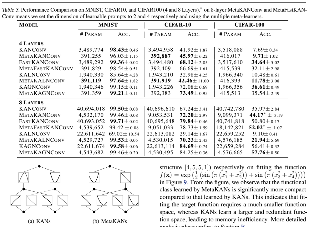
- [Section 3.2.2, Eq. (9); Table 1; Table 9] The paper's central parameter-count formula assumes a scalar prompt z in R, giving |Z| = sum_l (n_l n_{l+1}) and meta-learner cost C*(d_hidden+1)*(G+k+1). However, Section 4.2.1 states that the 8-layer MetaKANConv and MetaFastKANConv used in Table 3 set the prompt dimension to 2 and 4, and Table 9 shows that the best CIFAR-100 accuracies occur at dim_z=2 or 4 (e.g., MetaFastKAN at C=7 improves from 44.16% at dim_z=1 to 52.02% at dim_z=4, with parameters increasing from 4,576,073 to 18,140,617). For dim_z=d, the prompt term should be d * sum_l (n_l n_{l+1}) and the meta-learner input layer has d*d_hidden additional parameters, so the formulas in Table 1 and Section 3.2.2 are not applicable to the reported best configurations. The headline '1/3 to 1/9 parameters' claim therefore needs to be restated with the correct dimension-dependent formula, and the main text should explain when the scalar special case is actually used.
- [Section 3.4] The stated condition for memory efficiency is algebraically reversed. With S = sum_l (n_l n_{l+1}) and m = G+k+1, MetaKAN has S + C(d_hidden+1)m parameters and KAN has mS. Requiring MetaKAN < KAN gives (d_hidden+1)m < (m-1)S, i.e., d_hidden+1 < (G+k)/(G+k+1) * S, not d_hidden ≳ (G+k)/(G+k+1) * S as written. Since this inequality is the paper's explicit justification for when MetaKAN improves memory efficiency, the error should be corrected and the surrounding discussion adjusted accordingly.
- [Table 8] In the 100-dimensional Allen-Cahn row, both KAN and MetaKAN are listed with 47,520 parameters. This is inconsistent with the method: for the structure [100,32,32,32,1], the KAN count equals (100*32 + 32*32 + 32*32 + 32*1)*(G+k+1) = 5,280*9, and a MetaKAN with any reasonable meta-learner should have far fewer than 47,520 parameters (the neighboring 100D rows report 6,697). The identical count suggests a typo or a misconfigured meta-learner, and it directly undermines the PDE parameter-efficiency claim in Table 8. The entry needs to be corrected or, if 47,520 is genuinely the value, the configuration and formula must be explained.
minor comments (6)
- [Section 3.2.1, heading] The heading contains a typo: 'UNDERSTANING' should be 'UNDERSTANDING'.
- [Eq. (12)] The loss expression 'ℓ(MetaKAN(x;Z,θ)−f(x))' should be 'ℓ(MetaKAN(x;Z,θ), f(x))' to match the usual supervised-loss notation used elsewhere.
- [Algorithm 1, line 5] The line 'Compute the output of MetaKAN using Eq. (3.2.2)' references an equation number that does not exist; it should refer to Eq. (10) or the relevant forward formula.
- [Table 5] The FMNIST 32,32 row contains the stray text '85.81S'; this should be cleaned up.
- [Section 4.1.2] The text first says 'across 16 Feynman equations' and then reports 'lower MSE in 11 out of 17'; the counts should be made consistent.
- [Figure 10 caption] The caption says 'pairwise absolute distances' while the text discusses 'similarity'; clarify whether darker regions indicate smaller distance or higher similarity.
Circularity Check
No significant circularity: the parameter reduction is a counting identity and performance claims are benchmarked externally.
full rationale
The core derivation in Section 3.2.2 is not circular. Equation (9) posits a meta-learner M_theta: R -> R^{G+k+1}, and Eq. (10) replaces each KAN spline coefficient vector w with M_theta(z); the resulting parameter count |Z|+|Theta| = sum_l (n_l n_{l+1}) + C(d_hidden+1)(G+k+1) is an accounting identity, not a fitted quantity renamed as a prediction. The sufficiency of a scalar prompt is a modeling assumption that is tested empirically against KAN baselines on Feynman regression, PDEs, and image classification, and Section 3.4 explicitly states when the fixed meta-learner cost pays off, conceding small KANs may not benefit. Self-citations to the authors' earlier meta-learning papers (Shu et al.; Xu et al.) are motivational and do not carry the derivation. The skeptic's observation that the best CIFAR-100 configurations use dim(z)=2 or 4 rather than the scalar z of Eq. (9) is a consistency and overstatement concern about which configuration realizes the headline 1/3-to-1/9 parameter reduction, not a circular step; likewise, the prompt-similarity heatmap in Figure 10 is an interpretability sanity check rather than a load-bearing proof. Accordingly, no circular step can be exhibited.
Assumptions & free parameters
free parameters (4)
- meta-learner hidden dimension d_hidden =
32/64 (Feynman), per-dimension values from {8,16,32,32,64,64} (high-dim), {32,64,128} (classification)
- prompt dimension dim(z) =
1 by default; 2 and 4 in 8-layer ConvKAN experiments and ablation
- number of meta-learner clusters C =
1, 3, 5, or 7 depending on layer grouping
- meta-learner learning rate and prompt learning rate =
eta_1 in {1e-4, 1e-3}, eta_2 in {1e-3, 1e-2}
assumptions (5)
- standard math Kolmogorov-Arnold representation theorem: any continuous multivariate function can be written as a finite superposition of univariate functions.
- ad hoc to paper A scalar task prompt z per activation is sufficient to identify the correct univariate function within a shared functional class.
- domain assumption A two-layer MLP meta-learner is expressive enough to capture the shared weight-generation rule for all activations in a layer or cluster.
- ad hoc to paper Layer clusters derived by KMeans on output-channel sizes group layers with similar weight-generation rules.
- domain assumption Reducing trainable parameter count translates directly into reduced peak GPU memory during training.
invented entities (1)
-
learnable task prompt z per activation
Cite this review
Pith. "Pith review of Improving Memory Efficiency for Training KANs via Meta Learning." pith.science (2026). https://pith.science/paper/3J2JKOJR
@misc{pith2026250607549,
  author       = {Pith},
  title        = {Pith review of: Improving Memory Efficiency for Training KANs via Meta Learning},
  year         = {2026},
  howpublished = {\url{https://pith.science/paper/3J2JKOJR}},
  note         = {Machine review of arXiv:2506.07549}
}
read the original abstract
Inspired by the Kolmogorov-Arnold representation theorem, KANs offer a novel framework for function approximation by replacing traditional neural network weights with learnable univariate functions. This design demonstrates significant potential as an efficient and interpretable alternative to traditional MLPs. However, KANs are characterized by a substantially larger number of trainable parameters, leading to challenges in memory efficiency and higher training costs compared to MLPs. To address this limitation, we propose to generate weights for KANs via a smaller meta-learner, called MetaKANs. By training KANs and MetaKANs in an end-to-end differentiable manner, MetaKANs achieve comparable or even superior performance while significantly reducing the number of trainable parameters and maintaining promising interpretability. Extensive experiments on diverse benchmark tasks, including symbolic regression, partial differential equation solving, and image classification, demonstrate the effectiveness of MetaKANs in improving parameter efficiency and memory usage. The proposed method provides an alternative technique for training KANs, that allows for greater scalability and extensibility, and narrows the training cost gap with MLPs stated in the original paper of KANs. Our code is available at https://github.com/Murphyzc/MetaKAN.
Figures


Figures from the paper (7 more)


Reference graph
Works this paper leans on
-
[1]
Aghaei, A. A. rkan: Rational kolmogorov-arnold networks. arXiv preprint arXiv:2406.14495,
-
[2]
Accuracy improvements of 3.2-14.6 percentage points on small-to-large datasets. These outcomes validate meta-learner’s capability to achieve ef- fective balance between parameter reduction and accuracy maintenance across varied basis function implementations (B-spline basis, wavelet and RBF) and architectural depths. C.3. Solving PDEs C.3.1. EXPERIMENTALS...
work page 2024
-
[4]
Kagnns: Kolmogorov-arnold networks meet graph learning.arXiv preprint arXiv:2406.18380,
Bresson, R., Nikolentzos, G., Panagopoulos, G., Chatzianas- tasis, M., Pang, J., and Vazirgiannis, M. Kagnns: Kolmogorov-arnold networks meet graph learning.arXiv preprint arXiv:2406.18380,
-
[5]
Brown, T. B., Mann, B., Ryder, N., Subbiah, M., Kaplan, J., Dhariwal, P., Neelakantan, A., Shyam, P., Sastry, G., Askell, A., et al. Language models are few-shot learners. InProceedings of the 34th International Conference on Neural Information Processing Systems, pp. 1877–1901,
work page 1901
-
[7]
demonstrate mother function-dependent performance, with Mexican Hat wavelet achieving 73.62% accuracy on SVHN compared to 66.13% for DoG wavelet in MetaWavKAN. The dual-hidden-layer configuration improves generalization on CIFAR-10, where MetaWavKAN reaches 49.52% accuracy versus 46.34% in 15 Table 6.Classification accuracies and parameter counts for Fast...
-
[8]
Genet, R. and Inzirillo, H. Tkan: Temporal kolmogorov- arnold networks.arXiv preprint arXiv:2405.07344,
-
[9]
From the figure, we observe that the function class learned by MetaKANs is significantly more compact compared to that learned by KANs. This indicates that MetaKANs require a smaller set of function class to fit the target function, whereas KANs learn a relatively larger and redundant function class, leading to memory inefficiency. For KANs, it achieves t...
work page 2024
-
[10]
Huang, S., Zhao, Z., Li, C., and Bai, L. Timekan: Kan- based frequency decomposition learning architecture for long-term time series forecasting.arXiv preprint arXiv:2502.06910,
Show all 26 references
-
[11]
U-kan makes strong backbone for medi- cal image segmentation and generation.arXiv preprint arXiv:2406.02918,
Li, C., Liu, X., Li, W., Wang, C., Liu, H., Liu, Y ., Chen, Z., and Yuan, Y . U-kan makes strong backbone for medi- cal image segmentation and generation.arXiv preprint arXiv:2406.02918,
-
[12]
Kolmogorov-arnold networks are radial basis function networks.arXiv preprint arXiv:2405.06721,
Li, Z. Kolmogorov-arnold networks are radial basis function networks.arXiv preprint arXiv:2405.06721,
-
[13]
Y ., and Tegmark, M
Liu, Z., Wang, Y ., Vaidya, S., Ruehle, F., Halver- son, J., Solja ˇci´c, M., Hou, T. Y ., and Tegmark, M. Kan: Kolmogorov-arnold networks.arXiv preprint arXiv:2404.19756,
-
[18]
W., Liu, Z., and Hou, T
Wang, Y ., Siegel, J. W., Liu, Z., and Hou, T. Y . On the expressiveness and spectral bias of kans.arXiv preprint arXiv:2410.01803,
-
[19]
and Wang, X
Yang, X. and Wang, X. Kolmogorov-arnold transformer. arXiv preprint arXiv:2409.10594,
-
[20]
doi: https://doi.org/10.1016/j.jcp.2022.111232
ISSN 0021-9991. doi: https://doi.org/10.1016/j.jcp.2022.111232. URL https://www.sciencedirect.com/ science/article/pii/S0021999122002947. Zhang, X. and Zhou, H. Generalization bounds and model complexity for kolmogorov-arnold networks.arXiv preprint arXiv:2410.08026,
2022
-
[21]
Meta-learning via hypernetworks
Zhao, D., Kobayashi, S., Sacramento, J., and von Oswald, J. Meta-learning via hypernetworks. In4th Workshop on Meta-Learning at NeurIPS 2020 (MetaLearn 2020). NeurIPS,
2020
-
[22]
Unlike conventional convolution kernels, Kolmogorov- Arnold (KA) kernels consist of a set of univariate non- linear learnable activation functions
and extended by (Drokin, 2024), which replace traditional convolutional activation functions with Kolmogorov-Arnold-based transformations, such as spline (2), RBF (18), or wavelet (17). Unlike conventional convolution kernels, Kolmogorov- Arnold (KA) kernels consist of a set o...
2024
-
[24]
vs 9,011). This efficiency advantage amplifies with dimen- sionality - for the radial function f3, MetaKAN’s parameter count grows 28× from 10D to 1000D (97 to 2,759) versus KAN’s 89× increase (101 to 9,011), enabling MetaKAN to limit error growth to 26.8× compared to KAN’s 65...
-
[1989]
Kolmogorov-arnold convolutions: Design principles and empirical studies.arXiv preprint arXiv:2407.01092,
Drokin, I. Kolmogorov-arnold convolutions: Design principles and empirical studies.arXiv preprint arXiv:2407.01092,
-
[1990]
Kaa: Kolmogorov-arnold attention for enhancing attentive graph neural networks.arXiv preprint arXiv:2501.13456,
Fang, T., Gao, T., Wang, C., Shang, Y ., Chow, W., Chen, L., and Yang, Y . Kaa: Kolmogorov-arnold attention for enhancing attentive graph neural networks.arXiv preprint arXiv:2501.13456,
-
[1997]
Kac: Kolmogorov-arnold classifier for continual learning.arXiv preprint arXiv:2503.21076,
Hu, Y ., Liang, Z., Yang, F., Hou, Q., Liu, X., and Cheng, M.-M. Kac: Kolmogorov-arnold classifier for continual learning.arXiv preprint arXiv:2503.21076,
-
[2019]
Small sample learning in big data era.arXiv preprint arXiv:1808.04572,
Shu, J., Xu, Z., and Meng, D. Small sample learning in big data era.arXiv preprint arXiv:1808.04572,
-
[2020]
F., and Sacra- mento, J
von Oswald, J., Henning, C., Grewe, B. F., and Sacra- mento, J. Continual learning with hypernetworks. In 8th International Conference on Learning Representa- tions (ICLR 2020)(virtual). International Conference on Learning Representations,
2020
-
[2021]
Finding local diffusion schr\” odinger bridge using kolmogorov-arnold network.arXiv preprint arXiv:2502.19754,
Qiu, X., Yang, M., Ma, X., Li, F., Liang, D., Luo, G., Wang, W., Wang, K., and Li, S. Finding local diffusion schr\” odinger bridge using kolmogorov-arnold network.arXiv preprint arXiv:2502.19754,
-
[2022]
D., Tepsich, A
Bodner, A. D., Tepsich, A. S., Spolski, J. N., and Pourteau, S. Convolutional kolmogorov-arnold networks.arXiv preprint arXiv:2406.13155,
-
[2023]
Chebyshev polynomial-based kolmogorov-arnold networks: An efficient architecture for nonlinear function approximation.arXiv preprint arXiv:2405.07200,
SS, S., AR, K., KP, A., et al. Chebyshev polynomial-based kolmogorov-arnold networks: An efficient architecture for nonlinear function approximation.arXiv preprint arXiv:2405.07200,
-
[2024]
and Chen, H
Bozorgasl, Z. and Chen, H. Wav-kan: Wavelet kolmogorov- arnold networks.arXiv preprint arXiv:2405.12832,
Reviewed August 7, 2026 · model on record in the stance chip above.
Discussion (0). Sign in to comment.