SpINRv2: Implicit Neural Representation for Passband FMCW Radars

Harshvardhan Takawale; Nirupam Roy

REVIEW 4 major objections 6 minor 26 references

SpINRv2: Implicit Neural Representation for Passband FMCW Radars

T0 review · 4 major / 6 minor · reviewed 2026-08-07 · deepseek-v4-flash

Challenge this review Re-run · record.json Download PDF Read on arXiv ↗

Pith's one-line read SpINRv2 claims that FMCW radar volume reconstruction should be supervised directly on the complex frequency spectrum through a differentiable closed-form forward model, with sparsity and smoothness priors to resolve sub-bin phase ambiguity.

desk verdict A sensible frequency-domain forward model for FMCW radar INR, but the headline claim about high-frequency performance is exactly the part that goes untested. read the letter →

arxiv 2506.08163 v2 pith:AVWAQNKA submitted 2025-06-09 cs.CV

Harshvardhan Takawale , Nirupam Roy This is my paper

classification cs.CV

keywords FMCWradarimplicitneuralrepresentationfrequency-domainforwardmodelvolumetricreconstructionspectralleakagephasealiasingsparsityregularizationmmWave

verification ladder T0 review T1 audit T2 compute T3 formal

The pith

A machine-rendered reading of the paper's core claim, the machinery that carries it, and where it could break.

The reading

SpINRv2 claims that high-fidelity 3D volume reconstruction from FMCW radar is best done by supervising an implicit neural field directly in the frequency domain, using a closed-form differentiable model of the complex beat spectrum instead of simulating time-domain waveforms. The paper argues that time-domain supervision is ill-conditioned because tiny range shifts scramble the oscillating beat signal, and that naive frequency-domain shortcuts such as range quantization throw away spectral leakage and phase information. SpINRv2 synthesizes only the DFT bins that correspond to valid scene ranges, adds sparsity and smoothness priors to resolve sub-bin phase ambiguities, and reports better IoU, chamfer distance, PSNR, SSIM, and LPIPS than backprojection and learning-based baselines on synthetic cylindrical-aperture scenes. The claim matters because if it holds, neural radar imaging can move from coarse voxel grids to continuous scattering fields with less computation and better high-frequency behavior.

What carries the argument

The load-bearing object is a closed-form spectral synthesis formula: for a scatterer at point $x$ with round-trip delay $\tau(x)$, the complex response at DFT bin $k$ is an integral over the scene of $\sigma(x)$ times a propagation factor and a Dirichlet-kernel leakage term, with phase $\phi(x) = 2\pi f_0\tau(x)$ set by the chirp start frequency. This formula lets the model compute only the $K$ frequency bins that correspond to valid scene delays, avoiding full time-domain simulation and FFT, and it keeps the forward map fully differentiable. Paired with an implicit neural representation for the scattering field $\sigma(x)$, plus $\ell^1$ sparsity and local smoothness regularizers, the mechanism turns FMCW spectral measurements into a continuous volumetric reconstruction.

What would settle it

Run the identical reconstruction pipeline with the chirp start frequency set to 77 GHz, or an equivalent simulation where $\lambda/4$ is about a millimetre and well below the bin resolution, and measure IoU and chamfer distance against the same baselines; if the reported gap closes or shell artifacts persist despite regularization, the high-frequency claim does not cover the intended mmWave regime.

Watch

Extended reading notes

Core claim

On its own terms, the paper's central discovery is that the FMCW beat signal's DFT has a closed form in terms of round-trip delay and chirp parameters, so the radar forward model can be evaluated directly at relevant frequency bins and supervised against complex measurements. The resulting system, SpINRv2, represents the scene as an implicit neural field predicting scatterer intensity and trains it with a magnitude and complex-component spectral loss plus smoothness and sparsity regularization. The paper reports that this combination outperforms time-domain simulation, range quantization, and coherent backprojection across all six metrics it evaluates, and degrades gracefully as bandwidth shrinks from 4 GHz to 40 MHz. It also reports that the high start-frequency regime is where the gap is largest, provided the regularizers are present.

Load-bearing premise

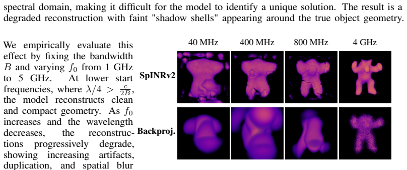
The paper tests start frequencies only from 1 to 5 GHz, far below the 76-81 GHz band of the mmWave sensor it mimics, and gives no reason the results would carry over to that more severe phase-wrapping regime.

Editorial extensions

If this is right

Frequency-domain supervision replaces time-domain MSE, which should make neural radar reconstruction trainable where time-domain losses plateau or explode.
Because only the bins inside the scene's delay range are computed, forward passes become cheaper than full 256-sample simulation plus FFT; the paper reports a runtime advantage that grows with scene size.
The closed-form leakage model captures sub-bin energy spill, so scatterers no longer need to align with bin centers for accurate reconstruction.
Smoothness and sparsity regularizers suppress the shell artifacts that appear when $\lambda/4 < c/(2B)$, extending the usable start-frequency range.
The continuous INR representation degrades gracefully under low bandwidth down to 40 MHz, unlike voxel-based backprojection which blurs sharply.

Reading between the lines

Editorial extensions of the paper, not claims the author makes directly.

A direct test the paper leaves open is whether the same gains appear at true automotive mmWave frequencies of 76-81 GHz: the experiments stop at 5 GHz, where $\lambda/4$ is roughly 15 mm, while at 77 GHz it is roughly 1 mm, a far harsher aliasing regime.
The frequency-domain forward model could be lifted to other coherent modalities that produce complex spectra, such as stepped-frequency radar or FMCW LiDAR, wherever the measurement is a Fourier transform over delay.
The staged loss schedule, magnitude first and then real and imaginary components, hints at a coarse-to-fine spectral supervision strategy that may benefit other inverse problems in sonar or ultrasound.
Because the experimental setup is a synthetic aperture, extending SpINRv2 with motion estimation could open the way to dynamic scenes, a direction the paper lists as future work but does not explore.

Share X Bluesky LinkedIn Reddit HN

Editorial analysis

A structured set of objections, weighed in public.

Desk editor's note, referee report, and a circularity audit.

Desk Editor's Note

read the letter

Quick take: the core idea is legitimate and the forward-model math is clean, but the paper's central claim is the one thing it never actually tests. The frequency-domain synthesis is a textbook DFT of a delayed chirp, but putting it inside an INR with spectral supervision on only the relevant bins is a sensible and modestly new combination, and the efficiency argument (skip full time-domain simulation and FFT) holds in the synthetic setup. I credit the authors for the closed-form leakage treatment and for ablating the regularization terms.

The soft spots are load-bearing. First, the evaluation is entirely generated with the same noiseless isotropic point-scatterer model the forward model encodes, so it is a round-trip simulation test, not evidence about physical fidelity. No noise, no error bars, no hardware. Second, the "high start frequencies" claim is tested only up to f0 = 5 GHz with B = 3.585 GHz, so f0/B is at most about 1.4, while the motivating AWR1843BOOST operates near 77 GHz with f0/B around 21. The phase-aliasing regime they say is central is extrapolated by an order of magnitude, and their own sheet benchmark (Fig. 13) shows degradation at fine detail, which does not make the extrapolation reassuring. Third, the multistatic-to-monostatic transformation is asserted but never specified, and the data normalization is vague. Fourth, they cite their prior SpINR in the abstract but omit it from the references, so the delta over prior work cannot be checked. That last one is sloppy but fixable.

The paper is not a waste of time. If the authors run the method at true mmWave parameters, add noise and clutter, specify the transformation, and release code, it could become a credible benchmark. As is, I would not accept the strong claims, but I would still send it to peer review: the method is coherent, the math is internally consistent, and the evaluation can be fixed in a major revision. My guess is reviewers will want realistic or real data before believing the "new benchmark" line.

Referee Report

4 major / 6 minor

Summary. The paper proposes SpINRv2, an implicit neural representation framework for volumetric FMCW radar reconstruction. It derives a closed-form frequency-domain forward model from the DFT of a dechirped beat signal, supervises the complex spectrum directly, and adds smoothness and sparsity regularizers. The method is evaluated on synthetic cylindrical-aperture data against time-domain, range-quantized, and backprojection baselines, with reported gains in IoU, Chamfer distance, Hausdorff distance, PSNR, SSIM, LPIPS, and runtime. The central claim is that the approach works under high start frequencies, where phase aliasing and sub-bin ambiguity become prominent.

Significance. The closed-form differentiable spectral synthesis is a useful idea that, if correct and properly validated, could improve both the stability and efficiency of neural radar reconstruction relative to time-domain simulation plus FFT. Explicitly modeling spectral leakage and using sparsity/smoothness priors are sensible design choices. However, the current evidence does not establish the paper's stronger claims: all measurements are simulated under the same ideal point-scatterer, noiseless, occlusion-free assumptions embodied by the forward model, and the 'high start frequency' regime is tested at carrier frequencies an order of magnitude below the motivating hardware. The absence of error bars, code, or real data further limits the claim of a new benchmark.

major comments (4)

[Section 4.2] The DFT synthesis formula is dimensionally inconsistent as written. For the sampled beat signal b(nTs)=exp(j2π f0 τ) exp(j2π S τ n Ts), the per-sample phase increment is 2π S τ / Fs, where Fs is the sampling rate. The display equation in Section 4.2 instead uses 2π S τ(x) in the numerator and subtracts β_k = 2πk/N from it. This mixes a frequency in Hz with an angle in radians and is not a valid DFT of the sampled chirp. Since the synthetic measurements in Section 5 are generated by a time-domain simulation followed by DFT, the reported experiments can be internally self-consistent even if this equation is not physically correct. Please correct the formula (including the 1/Fs or Ts factor) and confirm that the implementation matches the corrected expression.
[Section 6.5.3 and Abstract] The central 'high start frequency' claim is not tested in the regime that motivates it. The ablation fixes B=3.585 GHz and varies f0 only from 1 GHz to 5 GHz, so the dimensionless parameter f0/B reaches at most 1.39 and λ/4 is no smaller than about 15 mm. The TI AWR1843BOOST hardware cited in Section 5 operates at 76–81 GHz, for which f0/B ≈ 21.5 and λ/4 ≈ 1 mm against a range bin of about 41.8 mm. Phase aliasing is therefore an order of magnitude more severe than anything evaluated, and the paper gives no scaling argument for why behavior at 1–5 GHz carries over to 77 GHz. The sentence 'SpINRv2 works under high start frequencies—where phase aliasing and sub-bin ambiguity become prominent' is consequently unsupported by the reported experiments.
[Section 5 and Section 6] The evaluation is entirely synthetic and is generated from the same ideal point-scatterer assumptions that the forward model encodes. Section 5 describes a noiseless simulation of 691,200 multistatic measurements followed by a multistatic-to-monostatic transformation, but the transformation is not specified and is not validated against true multistatic or real-world data. There is no test with noise, clutter, occlusion, multipath, non-point scatterers, or the antenna patterns of actual mmWave hardware. Tables 1 and 2 report point estimates without error bars or significance tests, so the statement that SpINRv2 'significantly outperforms' the baselines is not statistically grounded. A real-radar validation (even limited) or a clearly stated restriction of the claims to the simulated ideal scenario is needed before the 'new benchmark' claim can be accepted.
[Sections 4.3 and 6.5.5] The optimization procedure is incompletely specified. Section 4.3 defines a fixed total loss with weights β and γ, but Section 6.5.5 introduces a staged supervision schedule in which the abs-term is used alone for the first 10% of transmitter locations and the complex terms are added later. This schedule is not part of the loss definition in Section 4, and the manuscript does not report values for β, γ, ε, the stage duration, or the switch criterion. Because these choices directly affect all reported reconstructions, they are load-bearing for reproducibility.

minor comments (6)

[Section 5] The word 'commertial' should be 'commercial'.
[Section 3.2] The notation 'm(t) ∗ ˆm(t)' should be multiplication, not convolution; the beat-signal derivation is otherwise described in words as mixing.
[Section 6.5.3] The text says f0 is varied from 1 GHz to 5 GHz, but Figure 10 caption lists only 2, 3, and 4 GHz; please reconcile the experimental range and the figure.
[Section 6.5.3] The sentence 'In the next section we show how regularization helps with higher frequencies' is inaccurate: the next section is the high-frequency sheet benchmark, while regularization is the topic of Section 6.5.1.
[Table 1] The PSNR entry for TF-SS is given as 13.5134 with excessive and inconsistent decimal places; use uniform formatting across all entries.
[Section 6] The baseline list says 'All methods are trained' but coherent backprojection is not trained; please rephrase to distinguish learned baselines from the classical method.

Circularity Check

1 steps flagged · score 4.0 of 10

The closed-form forward model is a genuine first-principles DFT derivation, but the synthetic measurements are generated from the same delayed-tone model, so the empirical benchmark is self-referential rather than independently validating.

other [Section 4.2 Spectral Synthesis vs. Section 5 Experimental Setup (data generation)]
"Zk = M N eiϕ · 1 − eiαN 1 − ei(α−βk) (Eq. 1); ... Our radar simulation follows the commertial TI AWR1843BOOST MIMO configuration, with a 3.585 GHz bandwidth, 70.295 × 1012 Hz/s chirp slope, and a sampling rate of5 MHz, yielding 256 ADC samples per chirp. These time-domain beat signals are transformed via DFT into 256 frequency bins as discussed in Section 4.1."

The ground-truth spectra are the DFT of time-domain beat signals modeled in Section 3.2 as b(t)=σ e^{j2πf0τ} e^{j2πSτ t}. Equation (1) is exactly the DFT of that delayed complex exponential, and Section 4.2 substitutes α=2πSτ and φ=2πf0τ to obtain Z_k. Thus the supervision targets lie in the forward model's own function class by construction: the data are generated from the same noiseless delayed-tone assumptions the model encodes. Optimizing the INR against these targets therefore validates inversion of the authors' own generative model, not agreement with independent FMCW radar physics. The derivation itself is not circular, but the empirical 'new benchmark' claim rests on a self-referential evaluation loop.

full rationale

No load-bearing self-citation was found: the prior SpINR is mentioned but not cited, and the derivation of Z_k from the DFT of a delayed tone is self-contained and parameter-free. No fitted parameter is renamed as a prediction, and no uniqueness theorem is imported from the authors' prior work. The one circularity-like element is the evaluation: synthetic measurements are produced by DFT of simulated beat signals whose analytic DFT is the paper's forward model, so the reported gains over baselines demonstrate self-consistency within the model's assumptions rather than physical fidelity. Because the forward-model derivation itself is not circular, this is partial rather than total circularity.

Assumptions & free parameters 5 free parameters · 5 assumptions · 0 invented entities

The method has no fitted physical constants, but it relies on several clean-scene assumptions: isotropic point scatterers, noiseless propagation, and a lossless multistatic-to-monostatic normalization. The experimental transfer from 1-5 GHz to mmWave is an unverified ad hoc assumption. The most consequential unstated items are the regularization weights and the INR architecture, which are not reported.

free parameters (5)

lambda (magnitude vs complex loss weight) = 0.5
Set by hand in Section 4.2; controls the balance between magnitude and phase supervision.
beta (smoothness regularization weight)
Introduced in Section 4.3 as a tunable weight; no value is reported in the text.
gamma (sparsity regularization weight)
Introduced in Section 4.3 as a tunable weight; no value is reported.
epsilon (smoothness perturbation scale)
The smoothness loss samples offsets delta_x ~ U(-epsilon, epsilon)^3 in Section 4.3; epsilon is not specified.
staged supervision schedule = 10% of transmitter locations
Section 6.5.5: magnitude-only loss is applied for the first 10% of transmitter locations before switching to the combined loss.

assumptions (5)

standard math DFT of a finite complex exponential has the closed form Z_k = (M/N) e^{i phi} (1 - e^{i alpha N}) / (1 - e^{i (alpha - beta_k)}).
Used in Eq. 1 (Section 4.1) as the basis for spectral synthesis.
domain assumption The FMCW beat signal after dechirping is a single complex exponential at angular frequency 2 pi S tau with phase 2 pi f0 tau, ignoring residual video phase.
Section 3.2, following Wang et al. 2014; the RVP term is neglected.
domain assumption The scene is a set of independent isotropic point scatterers with scalar reflectivity sigma(x); no occlusion, multipath, view-dependent reflectivity, or noise is modeled.
Section 4.2 forward model integrates sigma(x) over X with 1/(N RT RR) amplitude and coherent phase only.
domain assumption The multistatic-to-monostatic transformation applied to the 691,200 MIMO measurements is lossless and makes the data consistent with the single-transceiver forward model.
Section 5; the transformation is stated without derivation.
ad hoc to paper The simulated f0 sweep from 1 to 5 GHz is representative of the high-start-frequency passband regime of the TI AWR1843BOOST mmWave radar.
Section 6.5.3; no scaling argument connects these frequencies to the 76-81 GHz operating band.

how reviews work

0 comments

Cite this review

Pith. "Pith review of SpINRv2: Implicit Neural Representation for Passband FMCW Radars." pith.science (2026). https://pith.science/paper/AVWAQNKA

@misc{pith2026250608163,
  author       = {Pith},
  title        = {Pith review of: SpINRv2: Implicit Neural Representation for Passband FMCW Radars},
  year         = {2026},
  howpublished = {\url{https://pith.science/paper/AVWAQNKA}},
  note         = {Machine review of arXiv:2506.08163}
}

read the original abstract

We present SpINRv2, a neural framework for high-fidelity volumetric reconstruction using Frequency-Modulated Continuous-Wave (FMCW) radar. Extending our prior work (SpINR), this version introduces enhancements that allow accurate learning under high start frequencies-where phase aliasing and sub-bin ambiguity become prominent. Our core contribution is a fully differentiable frequency-domain forward model that captures the complex radar response using closed-form synthesis, paired with an implicit neural representation (INR) for continuous volumetric scene modeling. Unlike time-domain baselines, SpINRv2 directly supervises the complex frequency spectrum, preserving spectral fidelity while drastically reducing computational overhead. Additionally, we introduce sparsity and smoothness regularization to disambiguate sub-bin ambiguities that arise at fine range resolutions. Experimental results show that SpINRv2 significantly outperforms both classical and learning-based baselines, especially under high-frequency regimes, establishing a new benchmark for neural radar-based 3D imaging.

Figures

Figures reproduced from arXiv: 2506.08163 by the authors.

**Figure 2.** Loss calculated on Time domain signal vs. loss calculated on [PITH_FULL_IMAGE:figures/full_fig_p004_2.png] view at source ↗

**Figure 3.** Loss when λ/4 < ∆r vs. loss when λ/4 > ∆r. As the start frequency increases the loss landscaped becomes non-flat due to ambiguity. While our frequencydomain forward model analytically captures the spectral response of a scene, it introduces a key challenge: ambiguity within each range bin. In FMCW radar, the center frequency of each FFT bin corresponds to a specific round-trip delay, and hence to a shell of poss… view at source ↗

Figures from the paper (8 more)

**Figure 4.** Figure 4: Comparison of volumetric reconstructions for Range Quantization, Time-domain forward [PITH_FULL_IMAGE:figures/full_fig_p008_4.png]

**Figure 6.** Figure 6: Comparison of the three forward models for their runtime and volume reconstruction accuracy. Even though the Range Quantization has the fastest runtime, it severely underperforms in volume reconstruction as signified by the chamfer distance (lower better). 6.2 Imp…

**Figure 7.** Figure 7: Comparison between (a) Mean and (b) standard deviation of the gradients for the first [PITH_FULL_IMAGE:figures/full_fig_p010_7.png]

**Figure 8.** Figure 8: Effect of smoothness and sparsity regularization on reconstruction quality. Top row shows the 3D reconstruction for various objects and the bottom row shows a 2D slice plot of the same object. Regularization reduces noise, eliminates shell artifacts, and improves su…

**Figure 9.** Figure 9: Comparison of volumetric reconstructions for different [PITH_FULL_IMAGE:figures/full_fig_p013_9.png]

**Figure 10.** Figure 10: Effect of different start frequencies 2, 3, 4 GHz [PITH_FULL_IMAGE:figures/full_fig_p013_10.png]

**Figure 11.** Figure 11: Groundtruth 3D sheet geometry [PITH_FULL_IMAGE:figures/full_fig_p013_11.png]

**Figure 14.** Figure 14: Effect of noise level on MSE metrics across different components. As shown in [PITH_FULL_IMAGE:figures/full_fig_p014_14.png]

Discussion (0). Sign in to comment.

Reference graph

Works this paper leans on

26 extracted references · 20 canonical work pages

[1]

Fauzia Ahmad and Moeness G. Amin. Through-the-wall human motion indication using sparsity-driven change detection. IEEE Transactions on Geoscience and Remote Sensing, 51 0 (2): 0 881--890, 2013. doi:10.1109/TGRS.2012.2203310

work page arXiv 2013
[2]

A review of the state of the art and future challenges of deep learning-based beamforming

Haya Al Kassir, Zaharias D Zaharis, Pavlos I Lazaridis, Nikolaos V Kantartzis, Traianos V Yioultsis, and Thomas D Xenos. A review of the state of the art and future challenges of deep learning-based beamforming. IEEE Access, 10: 0 80869--80882, 2022

work page 2022
[3]

David Balduzzi, Marcus Frean, Lennox Leary, J P Lewis, Kurt Wan-Duo Ma, and Brian McWilliams. The shattered gradients problem: if resnets are the answer, then what is the question? In Proceedings of the 34th International Conference on Machine Learning - Volume 70, ICML'17, page 342–350. JMLR.org, 2017

work page 2017
[4]

Neural implicit surface reconstruction of freehand 3d ultrasound volume with geometric constraints

Hongbo Chen, Logiraj Kumaralingam, Shuhang Zhang, Sheng Song, Fayi Zhang, Haibin Zhang, Thanh-Tu Pham, Kumaradevan Punithakumar, Edmond HM Lou, Yuyao Zhang, et al. Neural implicit surface reconstruction of freehand 3d ultrasound volume with geometric constraints. Medical Image Analysis, 98: 0 103305, 2024

work page 2024
[5]

Highly accelerated mri via implicit neural representation guided posterior sampling of diffusion models, 2024

Jiayue Chu, Chenhe Du, Xiyue Lin, Yuyao Zhang, and Hongjiang Wei. Highly accelerated mri via implicit neural representation guided posterior sampling of diffusion models, 2024

work page 2024
[6]

Airsas: Controlled dataset generation for physics-informed machine learning

Benjamin Cowen, J Daniel Park, Thomas E Blanford, Geoff Goehle, and Daniel C Brown. Airsas: Controlled dataset generation for physics-informed machine learning. In NeurIPS Data-Centric AI Workshop, 2021

work page 2021
[7]

Backprojection for synthetic aperture radar

Michael Israel Duersch. Backprojection for synthetic aperture radar. Brigham Young University, 2013

work page 2013
[8]

Deep sar-net: Learning objects from signals

Zhongling Huang, Mihai Datcu, Zongxu Pan, and Bin Lei. Deep sar-net: Learning objects from signals. ISPRS Journal of Photogrammetry and Remote Sensing, 161: 0 179--193, 2020. ISSN 0924-2716. doi:https://doi.org/10.1016/j.isprsjprs.2020.01.016. URL https://www.sciencedirect.com/science/article/pii/S0924271620300162

work page doi:10.1016/j.isprsjprs.2020.01.016 2020

Show all 26 references

[9]

Depth estimation from monocular images and sparse radar using deep ordinal regression network

Chen-Chou Lo and Patrick Vandewalle. Depth estimation from monocular images and sparse radar using deep ordinal regression network. In 2021 IEEE International Conference on Image Processing (ICIP), pages 3343--3347, 2021. doi:10.1109/ICIP42928.2021.9506550

2021
[10]

Transient neural radiance fields for lidar view synthesis and 3d reconstruction

Anagh Malik, Parsa Mirdehghan, Sotiris Nousias, Kyros Kutulakos, and David Lindell. Transient neural radiance fields for lidar view synthesis and 3d reconstruction. Advances in Neural Information Processing Systems, 36: 0 71569--71581, 2023

2023
[11]

Srinivasan, Matthew Tancik, Jonathan T

Ben Mildenhall, Pratul P. Srinivasan, Matthew Tancik, Jonathan T. Barron, Ravi Ramamoorthi, and Ren Ng. Nerf: representing scenes as neural radiance fields for view synthesis. Commun. ACM, 65 0 (1): 0 99–106, December 2021. ISSN 0001-0782. doi:10.1145/3503250. URL https://doi-...

2021 doi
[12]

Papathanassiou

Alberto Moreira, Pau Prats-Iraola, Marwan Younis, Gerhard Krieger, Irena Hajnsek, and Konstantinos P. Papathanassiou. A tutorial on synthetic aperture radar. IEEE Geoscience and Remote Sensing Magazine, 1 0 (1): 0 6--43, 2013. doi:10.1109/MGRS.2013.2248301

2013
[13]

Automotive radars: A review of signal processing techniques

Sujeet Milind Patole, Murat Torlak, Dan Wang, and Murtaza Ali. Automotive radars: A review of signal processing techniques. IEEE Signal Processing Magazine, 34 0 (2): 0 22--35, 2017. doi:10.1109/MSP.2016.2628914

2017
[14]

Neural volumetric reconstruction for coherent synthetic aperture sonar

Albert Reed, Juhyeon Kim, Thomas Blanford, Adithya Pediredla, Daniel Brown, and Suren Jayasuriya. Neural volumetric reconstruction for coherent synthetic aperture sonar. ACM Trans. Graph., 42 0 (4), July 2023. ISSN 0730-0301. doi:10.1145/3592141. URL https://doi-org.proxy-um.r...

2023 doi
[15]

Radar-based perception for autonomous outdoor vehicles

Giulio Reina, James Underwood, Graham Brooker, and Hugh Durrant-Whyte. Radar-based perception for autonomous outdoor vehicles. J. Field Robot., 28 0 (6): 0 894–913, November 2011. ISSN 1556-4959. doi:10.1002/rob.20393. URL https://doi-org.proxy-um.researchport.umd.edu/10.1002/...

2011 doi
[16]

Deep learning-driven state correction: A hybrid architecture for radar-based dynamic occupancy grid mapping, 2024

Max Peter Ronecker, Xavier Diaz, Michael Karner, and Daniel Watzenig. Deep learning-driven state correction: A hybrid architecture for radar-based dynamic occupancy grid mapping, 2024

2024
[17]

Sankararaman, Soham De, Zheng Xu, W

Karthik A. Sankararaman, Soham De, Zheng Xu, W. Ronny Huang, and Tom Goldstein. The impact of neural network overparameterization on gradient confusion and stochastic gradient descent. In Proceedings of the 37th International Conference on Machine Learning, ICML'20. JMLR.org, 2020

2020
[18]

Vincent Sitzmann, Julien N. P. Martel, Alexander W. Bergman, David B. Lindell, and Gordon Wetzstein. Implicit neural representations with periodic activation functions. In Proceedings of the 34th International Conference on Neural Information Processing Systems, NIPS '20, Red ...

2020
[19]

Dynamic targets occupancy status detection utilizing mmwave radar sensor and ensemble machine learning

Amala Sonny, Abhinav Kumar, and Linga Reddy Cenkeramaddi. Dynamic targets occupancy status detection utilizing mmwave radar sensor and ensemble machine learning. IEEE Open Journal of the Industrial Electronics Society, 2024

2024
[20]

Wide-band range-doppler processing for fmcw systems

Thomas Wagner, Reinhard Feger, and Andreas Stelzer. Wide-band range-doppler processing for fmcw systems. In 2013 European Radar Conference, pages 160--163. IEEE, 2013

2013
[21]

Picking winning tickets before training by preserving gradient flow

Chaoqi Wang, Guodong Zhang, and Roger Grosse. Picking winning tickets before training by preserving gradient flow. In Proceedings of the 8th International Conference on Learning Representations (ICLR), 2020, 2020

2020
[22]

Application of linear-frequency-modulated continuous-wave (lfmcw) radars for tracking of vital signs

Guochao Wang, José-María Muñoz-Ferreras, Changzhan Gu, Changzhi Li, and Roberto Gómez-García. Application of linear-frequency-modulated continuous-wave (lfmcw) radars for tracking of vital signs. IEEE Transactions on Microwave Theory and Techniques, 62 0 (6): 0 1387--1399, 201...

2014
[23]

Learned depth estimation of 3d imaging radar for indoor mapping

Ruoyang Xu, Wei Dong, Akash Sharma, and Michael Kaess. Learned depth estimation of 3d imaging radar for indoor mapping. In 2022 IEEE/RSJ International Conference on Intelligent Robots and Systems (IROS), pages 13260--13267. IEEE, 2022

2022
[24]

Development and demonstration of mimo-sar mmwave imaging testbeds

Muhammet Emin Yanik, Dan Wang, and Murat Torlak. Development and demonstration of mimo-sar mmwave imaging testbeds. IEEE Access, 8: 0 126019--126038, 2020. doi:10.1109/ACCESS.2020.3007877

2020
[25]

Yegulalp

A.F. Yegulalp. Fast backprojection algorithm for synthetic aperture radar. In Proceedings of the 1999 IEEE Radar Conference. Radar into the Next Millennium (Cat. No.99CH36249), pages 60--65, 1999. doi:10.1109/NRC.1999.767270

1999
[26]

Fixup initialization: Residual learning without normalization

Hongyi Zhang, Yann N Dauphin, and Tengyu Ma. Fixup initialization: Residual learning without normalization. arXiv preprint arXiv:1901.09321, 2019

1901 arXiv

Pith tools

Reviewed August 7, 2026 · model on record in the stance chip above.

[1] [1]

Fauzia Ahmad and Moeness G. Amin. Through-the-wall human motion indication using sparsity-driven change detection. IEEE Transactions on Geoscience and Remote Sensing, 51 0 (2): 0 881--890, 2013. doi:10.1109/TGRS.2012.2203310

work page arXiv 2013

[2] [2]

A review of the state of the art and future challenges of deep learning-based beamforming

Haya Al Kassir, Zaharias D Zaharis, Pavlos I Lazaridis, Nikolaos V Kantartzis, Traianos V Yioultsis, and Thomas D Xenos. A review of the state of the art and future challenges of deep learning-based beamforming. IEEE Access, 10: 0 80869--80882, 2022

work page 2022

[3] [3]

David Balduzzi, Marcus Frean, Lennox Leary, J P Lewis, Kurt Wan-Duo Ma, and Brian McWilliams. The shattered gradients problem: if resnets are the answer, then what is the question? In Proceedings of the 34th International Conference on Machine Learning - Volume 70, ICML'17, page 342–350. JMLR.org, 2017

work page 2017

[4] [4]

Neural implicit surface reconstruction of freehand 3d ultrasound volume with geometric constraints

Hongbo Chen, Logiraj Kumaralingam, Shuhang Zhang, Sheng Song, Fayi Zhang, Haibin Zhang, Thanh-Tu Pham, Kumaradevan Punithakumar, Edmond HM Lou, Yuyao Zhang, et al. Neural implicit surface reconstruction of freehand 3d ultrasound volume with geometric constraints. Medical Image Analysis, 98: 0 103305, 2024

work page 2024

[5] [5]

Highly accelerated mri via implicit neural representation guided posterior sampling of diffusion models, 2024

Jiayue Chu, Chenhe Du, Xiyue Lin, Yuyao Zhang, and Hongjiang Wei. Highly accelerated mri via implicit neural representation guided posterior sampling of diffusion models, 2024

work page 2024

[6] [6]

Airsas: Controlled dataset generation for physics-informed machine learning

Benjamin Cowen, J Daniel Park, Thomas E Blanford, Geoff Goehle, and Daniel C Brown. Airsas: Controlled dataset generation for physics-informed machine learning. In NeurIPS Data-Centric AI Workshop, 2021

work page 2021

[7] [7]

Backprojection for synthetic aperture radar

Michael Israel Duersch. Backprojection for synthetic aperture radar. Brigham Young University, 2013

work page 2013

[8] [8]

Deep sar-net: Learning objects from signals

Zhongling Huang, Mihai Datcu, Zongxu Pan, and Bin Lei. Deep sar-net: Learning objects from signals. ISPRS Journal of Photogrammetry and Remote Sensing, 161: 0 179--193, 2020. ISSN 0924-2716. doi:https://doi.org/10.1016/j.isprsjprs.2020.01.016. URL https://www.sciencedirect.com/science/article/pii/S0924271620300162

work page doi:10.1016/j.isprsjprs.2020.01.016 2020