REVIEW 2 major objections 6 minor 1 cited by
NeurIPS 2024 ML4CFD Competition: Results and Retrospective Analysis
T0 review · 2 major / 6 minor · reviewed 2026-08-07 · deepseek-v4-flash
Pith's one-line read The ML4CFD competition's top entry, a mesh-morphing Gaussian process, scored above the reference OpenFOAM solver on the aggregate evaluation.
desk verdict A useful competition retrospective whose headline claim is currently unauditable because the final scoring thresholds are never disclosed. read the letter →
The pith
A machine-rendered reading of the paper's core claim, the machinery that carries it, and where it could break.
The reading
What carries the argument
The load-bearing object is the global score, a linear combination of three subscores (ML accuracy and speed-up, physics compliance, OOD generalization) in which each metric is binned at two thresholds into 0, 1, or 2 points before being averaged; the weights are $\alpha_{ML}=0.4$, $\alpha_{OOD}=0.3$, $\alpha_{PH}=0.3$, with accuracy weighted at 0.75 against speed-up at 0.25. This scoring function is what lets the paper claim a surrogate can 'outperform' a high-fidelity solver, so the binned-threshold design carries the entire ranking argument. On the method side, the MMGP pipeline carries the winning result: morphing aligns each mesh's wake, snapshot POD compresses fields, and independent Gaussian processes regress the generalized coordinates, with the zero-velocity boundary condition preserved automatically by the linear reconstruction.
What would settle it
Recompute the global score for the top submissions using several plausible threshold sets (for example, varying the reported T1/T2 values by ±20 percent) and check whether MMGP still outranks OpenFOAM and the other finalists; if the rank order changes, the claim that a surrogate outperformed the reference solver is an artifact of the chosen thresholds.
Extended reading notes
Core claim
The paper's central claim is that the first-place solution, MMGP, achieved a global score of 84.68 that exceeds the OpenFOAM reference's score of 82.5 on a weighted combination of accuracy, speed-up, physics compliance of lift and drag, and out-of-distribution generalization (Table 4, rank 1, Safran-Tech). The authors attribute this result not to a larger model but to a deterministic reparametrization pipeline — mesh morphing onto a common shape, finite element interpolation onto a common mesh, snapshot POD dimensionality reduction, and independent Gaussian process regressors per generalized coordinate — which converts variable-size CFD meshes into fixed-size low-dimensional embeddings. They report that the winning approach beat both deep learning surrogates and the CFD solver on aggregate metrics, and that all top methods explicitly encoded geometric structure.
Load-bearing premise
The entire ranking — including the claim that the top entry beats OpenFOAM — rests on hand-chosen thresholds and weights in the scoring function, whose final-edition values are not reported and whose sensitivity is not tested; if a different reasonable threshold set changed category memberships, the leaderboard and its conclusions would change.
Editorial extensions
If this is right
- If the claim holds, classical kernel-based surrogates should be treated as serious baselines for small-data PDE problems, not just deep learning.
- Geometric reparametrization (morphing) can matter more than architectural complexity when training data is scarce.
- The multi-criteria evaluation framework, with explicit physics and OOD categories, provides a template for comparing ML surrogates against traditional solvers in other engineering domains.
- Deep learning methods' larger speedups are under-rewarded by the scoring weights, so different weight choices could change which approach wins; the paper acknowledges this tradeoff.
- Future SciML competitions should adopt the paper's recommendations: hidden test sets, multiple baselines, and statistical re-evaluation of final rankings.
Reading between the lines
- A natural robustness test is to recompute the leaderboard over the full threshold and weight space; the paper does not report sensitivity of the rank order beyond the speed-up metric, so the headline claim may be threshold-dependent.
- The MMGP recipe — align geometries, compress, regress — could transfer to other non-parameterized geometric variability problems, such as patient-specific hemodynamics or turbomachinery.
- The paper's reported speedup ratios (300–600x for neural methods versus MMGP) imply an accuracy/speed Pareto frontier; a future competition could score on the frontier rather than a fixed linear combination.
- Combining MMGP's morphing with neural inference speed might yield a strictly dominant surrogate, a hybrid the authors mention only implicitly.
Editorial analysis
A structured set of objections, weighed in public.
Referee Report
Summary. This paper reports the results and retrospective analysis of the NeurIPS 2024 ML4CFD competition, which tasked participants with building surrogate models for steady incompressible RANS simulations of 2D airfoils from the AirfRANS dataset. The evaluation used the LIPS framework, combining ML accuracy and speed-up, physics compliance of lift and drag, and out-of-distribution generalization, aggregated into a single weighted global score. The paper describes the dataset and competition logistics, presents a leaderboard, and analyzes the four winning methods: MMGP (PCA with Gaussian processes and mesh morphing), OB-GNN (offset-based graph convolutions), MARIO (conditional neural fields), and GeoMPNN (geometry-aware message passing). The headline claim is that the MMGP entry achieved the highest global score (84.68), slightly above the OpenFOAM reference (82.5), and the authors draw design principles, particularly the importance of geometric inductive biases.
Significance. If the ranking is robust, this is a useful empirical benchmark: a non-deep-learning surrogate built on 103 scarce samples outperforms both deep learning surrogates and the reference CFD solver on a multi-criteria score. The paper has concrete strengths: it is based on a real competition with over 240 teams, the dataset is public, code links for the winning methods are provided, and the authors are transparent about several evaluation choices, including the definition of speed-up and training-cost issues (Appendix D.1). However, the central quantitative claim rests on an undisclosed threshold configuration for the scoring function, and there are internal inconsistencies in reported speed-up values. These issues currently limit the verifiability of the paper's main conclusions.
major comments (2)
- [Appendix B / Table 4 / Eq. (8)] The final-edition thresholds T1 and T2 that convert each metric into 0, 1, or 2 points are not reported. Eq. (8) and the worked example in Table 3 apply to the preliminary edition, and the text explicitly states that the criteria 'slightly evolved' for the new edition. Because the global score (Eq. 6) is a weighted sum of these binned sub-scores, the leaderboard in Table 4 cannot be recomputed from the manuscript. The margin between the top entry (Safran-Tech, 84.68) and OpenFOAM (82.5) is only 2.18 points, so a small shift in thresholds could change several metrics' category memberships and potentially invert the headline ordering. The only robustness check reported (Appendix D.1) varies the speed-up definition, not the thresholds or the weights. Please disclose the final T1/T2 values for every metric and provide a sensitivity analysis over thresholds and weights demonstrating that the MMGP-versus-OpenFOAM ordering and the top-four ordering are stable.
- [§4.2 / §6 / §3] The paper reports mutually inconsistent speed-up values for the same deep learning methods. Section 4.2 states that OB-GNN 'achieves a 7,000× speedup (220 ms vs 25 min per case),' Section 6 states that OB-GNN, MARIO, and GeoMPNN showed 'substantial computational speedups ranging from 300× to 600×,' and Section 3 states that the deep learning methods were 'typically 2–3× faster than MMGP.' These claims differ by orders of magnitude and cannot all describe the same evaluation. A single, consistent speed-up definition—preferably the competition metric in Eq. (11), which includes evaluation time—should be used throughout, and the reported numbers must be reconciled, since the paper's conclusions about the accuracy-speed trade-off depend on the correct order of magnitude.
minor comments (6)
- [Appendix B] There is a typo: 'everall score' should be 'overall score' in the Score Calculation Example.
- [Appendix E.5] There is a typo: 'seepdup' should be 'speedup'.
- [§4.3] There is a typo: 'distrbutions' should be 'distributions'.
- [Appendix E.2] There is a typo: 'ont of' should be 'one of'.
- [Appendix E.3] There is a typo: 'dimensionaly' should be 'dimensionality'.
- [Table 1] The sub-scores in Table 1 (e.g., '162.7 162.8' for MMGP) are not defined; Table 4 reports the same entry's ML/Physics/OOD sub-scores as 0.89/0.88/0.76. Please clarify the scaling and column headers so the two tables are consistent and interpretable.
Circularity Check
No circularity: the competition ranking is an evaluation result against held-out OpenFOAM ground truth; the undisclosed scoring thresholds are an auditability limitation, not a circular reduction.
full rationale
The paper is a competition retrospective rather than a derivation, and its load-bearing quantitative claims are empirical evaluation results, not consequences of fitted parameters renamed as predictions. Per-method accuracy, physics, and OOD sub-scores are computed against held-out OpenFOAM ground-truth fields (Section 2 and Appendix B), which is external evidence; the global score in Eq. (6) is a deterministic weighted sum of those external sub-scores. The headline that the top entry 'exceeded the performance of the original OpenFOAM solver on aggregate metrics' is explicitly qualified in the Abstract as holding 'under tailored criteria,' i.e., under the authors' stated scoring rule. That a ranking follows from the rule that defines it is tautological for any leaderboard, not a circularity in the sense of a prediction being equivalent to its inputs by construction. The main limitation is that the final-edition threshold values used in Eq. (8) are not reported, and Appendix B only gives a worked example for the 'preliminary edition,' noting the criteria 'slightly evolved.' This is a reproducibility and robustness weakness, but the paper does not hide the structure of the score, and no step in the paper fits a parameter to the quantity it then claims to predict. The self-citations ([14] LIPS, [19] competition design, [22] MMGP, [29] GeoMPNN) describe the platform and methods used, but the ranking evidence is presented in Tables 1 and 4 rather than imported from those references; even if those citations were removed, the evaluation results would stand as reported. No circular step satisfying the required quote-and-reduction standard can be exhibited, so the appropriate finding is no significant circularity.
Assumptions & free parameters
free parameters (4)
- scoring weights alpha_ML=0.4, alpha_OOD=0.3, alpha_PH=0.3, alpha_A=0.75, alpha_S=0.25 =
0.4 / 0.3 / 0.3 / 0.75 / 0.25 (preliminary; final values not fully specified)
- Accuracy thresholds T1/T2 per metric =
e.g., ux: 0.1/0.2; many final-edition values not disclosed
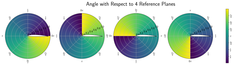
- SpeedUpMax cap =
10000 (preliminary example)
- MMGP POD mode counts and GP hyperparameters =
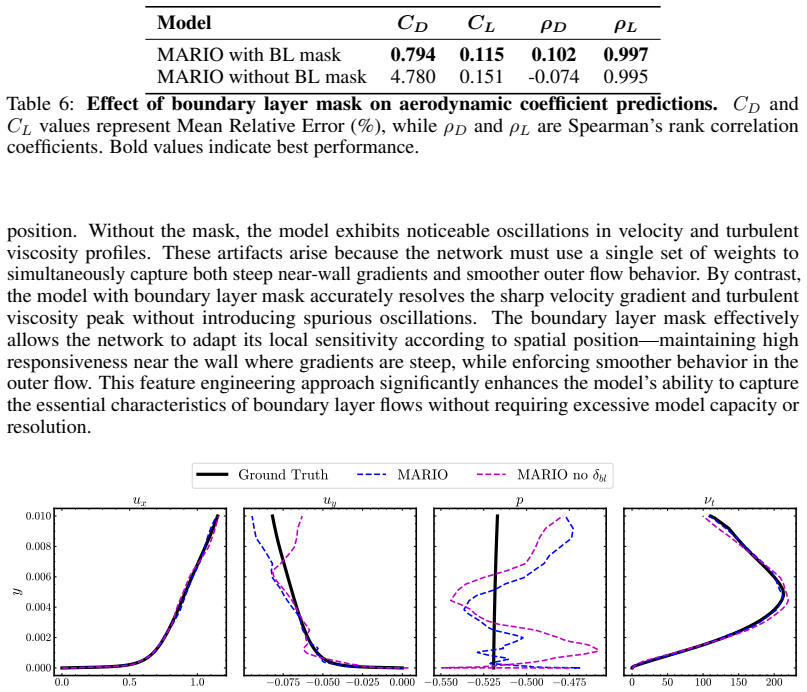
16 shape modes, 13 velocity, 24 pressure, 12 nu_t; RBF lengthscales, constant, noise fitted by AdamW
assumptions (4)
- domain assumption OpenFOAM simpleFOAM RANS (SST k-omega) solutions on C-meshes with y+ approx 1 are correct ground truth for the flow physics.
- ad hoc to paper Coarse 0/1/2-point binning with calibrated thresholds preserves the true performance ordering of methods.
- domain assumption CL/CD relative errors and Spearman correlations are sufficient physics-compliance criteria.
- domain assumption The data split (train Re in [3,5] x 10^6; OOD Re in [2,3] and [5,6] x 10^6) provides a valid test of inductive generalization.
Cite this review
Pith. "Pith review of NeurIPS 2024 ML4CFD Competition: Results and Retrospective Analysis." pith.science (2026). https://pith.science/paper/NGSDV4L2
@misc{pith2026250608516,
  author       = {Pith},
  title        = {Pith review of: NeurIPS 2024 ML4CFD Competition: Results and Retrospective Analysis},
  year         = {2026},
  howpublished = {\url{https://pith.science/paper/NGSDV4L2}},
  note         = {Machine review of arXiv:2506.08516}
}
read the original abstract
The integration of machine learning (ML) into the physical sciences is reshaping computational paradigms, offering the potential to accelerate demanding simulations such as computational fluid dynamics (CFD). Yet, persistent challenges in accuracy, generalization, and physical consistency hinder the practical deployment of ML models in scientific domains. To address these limitations and systematically benchmark progress, we organized the ML4CFD competition, centered on surrogate modeling for aerodynamic simulations over two-dimensional airfoils. The competition attracted over 240 teams, who were provided with a curated dataset generated via OpenFOAM and evaluated through a multi-criteria framework encompassing predictive accuracy, physical fidelity, computational efficiency, and out-of-distribution generalization. This retrospective analysis reviews the competition outcomes, highlighting several approaches that outperformed baselines under our global evaluation score. Notably, the top entry exceeded the performance of the original OpenFOAM solver on aggregate metrics, illustrating the promise of ML-based surrogates to outperform traditional solvers under tailored criteria. Drawing from these results, we analyze the key design principles of top submissions, assess the robustness of our evaluation framework, and offer guidance for future scientific ML challenges.
Figures


Figures from the paper (26 more)






Forward citations
Cited by 1 Pith paper
-
The HydroGym Reinforcement Learning Platform for Fluid Dynamics
HydroGym provides 42+ (abstract claims 61+) standardized RL environments for flow control, and reports policies that transfer across Reynolds numbers and geometries, including a 38% drag-reduction transfer claim not s...
Reference graph
Works this paper leans on
-
[1]
J. Tompson, K. Schlachter, P. Sprechmann, and K. Perlin. Accelerating eulerian fluid simulation with convolutional networks. ArXiv: 1607.03597, 2016
arXiv 2016
-
[2]
Building high accuracy emulators for scientific simulations with deep neural architecture search
MF Kasim, D Watson-Parris, L Deaconu, S Oliver, P Hatfield, DH Froula, G Gregori, M Jarvis, S Khatiwala, J Korenaga, et al. Building high accuracy emulators for scientific simulations with deep neural architecture search. Machine Learning: Science and Technology, 3(1):015013, 2021
work page 2021
-
[3]
S. Rasp, M. S. Pritchard, and P. Gentine. Deep learning to represent sub-grid processes in climate models. PNAS, 2018
work page 2018
-
[4]
Learning to simulate complex physics with graph networks
Alvaro Sanchez-Gonzalez, Jonathan Godwin, Tobias Pfaff, Rex Ying, Jure Leskovec, and Peter Battaglia. Learning to simulate complex physics with graph networks. In International Conference on Machine Learning, pages 8459–8468. PMLR, 2020
2020
-
[5]
Emmanuel Menier, Michele Alessandro Bucci, Mouadh Yagoubi, Lionel Mathelin, and Marc Schoenauer. Cd-rom: Complemented deep-reduced order model.Computer Methods in Applied Mechanics and Engineering, 410:115985, 2023
work page 2023
-
[6]
https://nips.cc/ virtual/2022/workshop/49979, 2022
Machine learning and the physical sciences workshop at neurips. https://nips.cc/ virtual/2022/workshop/49979, 2022
work page 2022
-
[7]
https://opencatalystproject.org/challenge.html, 2021- 2022
Open catalyst challenge. https://opencatalystproject.org/challenge.html, 2021- 2022
work page 2021
-
[8]
The higgs boson machine learning challenge
Claire Adam-Bourdarios, Glen Cowan, Cécile Germain, Isabelle Guyon, Balázs Kégl, and David Rousseau. The higgs boson machine learning challenge. In NIPS 2014 workshop on high-energy physics and machine learning, pages 19–55. PMLR, 2015
work page 2014
Show all 57 references
-
[9]
Adapt cascade competition: Sim2real object detection and pose-estimation challenge, 2023
2023
-
[10]
https://physics4ml.github.io/, 2023
Iclr 2023 workshop on physics for machine learning. https://physics4ml.github.io/, 2023
2023
-
[11]
Konstantin Rusch, and Siddhartha Mishra
Léonard Equer, T. Konstantin Rusch, and Siddhartha Mishra. Multi-scale message passing neural PDE solvers. In ICLR 2023 Workshop on Physics for Machine Learning, 2023
2023
-
[12]
Neural networks learn representation theory: Reverse engineering how networks perform group operations
Bilal Chughtai, Lawrence Chan, and Neel Nanda. Neural networks learn representation theory: Reverse engineering how networks perform group operations. In ICLR 2023 Workshop on Physics for Machine Learning, 2023
2023
-
[13]
Interpretable learning of effective dynamics for multiscale systems
Emmanuel Menier, Sebastian Kaltenbach, Mouadh Yagoubi, Marc Schoenauer, and Petros Koumoutsakos. Interpretable learning of effective dynamics for multiscale systems. In Proceedings A, volume 481, page 20240167. The Royal Society, 2025
2025
-
[14]
LIPS-learning industrial physical simulation benchmark suite
Milad Leyli-abadi, Antoine Marot, Jérôme Picault, David Danan, Mouadh Yagoubi, Benjamin Donnot, Seif Attoui, Pavel Dimitrov, Asma Farjallah, and Clement Etienam. LIPS-learning industrial physical simulation benchmark suite. Advances in Neural Information Processing Systems, 35...
2022
-
[15]
Applied computational aerodynamics
Daniel Livescu. Applied computational aerodynamics. a modern engineering approachcum- mingsrussell m.masonwilliam h.mortonscott a.mcdanieldavid r., cambridge university press, new york, 2015, 849 pp., 125.00. AIAA Journal, 54, 09 2016
2015
-
[16]
Airfrans: High fi- delity computational fluid dynamics dataset for approximating reynolds-averaged navier–stokes solutions
Florent Bonnet, Jocelyn Mazari, Paola Cinnella, and Patrick Gallinari. Airfrans: High fi- delity computational fluid dynamics dataset for approximating reynolds-averaged navier–stokes solutions. Advances in Neural Information Processing Systems, 35:23463–23478, 2022
2022
-
[17]
Kochkov, J
D. Kochkov, J. A. Smith, A. Alieva, and al. Machine learning–accelerated computational fluid dynamics. Proceedings of the National Academy of Sciences (PNAS), 2021
2021
-
[18]
Worrall, and Max Welling
Johannes Brandstetter, Daniel E. Worrall, and Max Welling. Message passing neural PDE solvers. In International Conference on Learning Representations, 2022. 10
2022
-
[19]
Neurips 2024 ml4cfd competition: Harnessing machine learning for computational fluid dynamics in airfoil design
Mouadh Yagoubi, David Danan, Milad Leyli-Abadi, Jean-Patrick Brunet, Jocelyn Ahmed Mazari, Florent Bonnet, Asma Farjallah, Paola Cinnella, Patrick Gallinari, Marc Schoenauer, et al. Neurips 2024 ml4cfd competition: Harnessing machine learning for computational fluid dynamics i...
2024 arXiv
-
[20]
Learn- ing mesh-based simulation with graph networks
Tobias Pfaff, Meire Fortunato, Alvaro Sanchez-Gonzalez, and Peter Battaglia. Learn- ing mesh-based simulation with graph networks. In International Conference on Learning Representations, 2021
2021
-
[21]
Multi-resolution graph neural networks for pde approximation
Wenzhuo Liu, Mouadh Yagoubi, and Marc Schoenauer. Multi-resolution graph neural networks for pde approximation. In Artificial Neural Networks and Machine Learning–ICANN 2021: 30th International Conference on Artificial Neural Networks, Bratislava, Slovakia, September 14–17, 20...
2021
-
[22]
MMGP: a Mesh Morphing Gaus- sian Process-based machine learning method for regression of physical problems under non- parametrized geometrical variability
Fabien Casenave, Brian Staber, and Xavier Roynard. MMGP: a Mesh Morphing Gaus- sian Process-based machine learning method for regression of physical problems under non- parametrized geometrical variability. Advances in Neural Information Processing Systems, 36, 2024
2024
-
[23]
Registration-based model reduction of parameterized pdes with spatio-parameter adaptivity
Nicolas Barral, Tommaso Taddei, and Ishak Tifouti. Registration-based model reduction of parameterized pdes with spatio-parameter adaptivity. Journal of Computational Physics, 499:112727, 2024
2024
-
[24]
Pointconv: Deep convolutional networks on 3d point clouds
Wenxuan Wu, Zhongang Qi, and Li Fuxin. Pointconv: Deep convolutional networks on 3d point clouds. In Proceedings of the IEEE/CVF Conference on computer vision and pattern recognition, pages 9621–9630, 2019
2019
-
[25]
Neural fields for rapid aircraft aerodynamics simulations
Giovanni Catalani, Siddhant Agarwal, Xavier Bertrand, Frédéric Tost, Michael Bauerheim, and Joseph Morlier. Neural fields for rapid aircraft aerodynamics simulations. Scientific Reports, 14(1):25496, 2024
2024
-
[26]
Geometry aware inference of steady state pdes using equivariant neural fields representations
Giovanni Catalani, Michael Bauerheim, Frédéric Tost, Xavier Bertrand, and Joseph Morlier. Geometry aware inference of steady state pdes using equivariant neural fields representations. arXiv preprint arXiv:2504.18591, 2025
2025
-
[27]
In- finity: Neural field modeling for reynolds-averaged navier-stokes equations
Louis Serrano, Leon Migus, Yuan Yin, Jocelyn Ahmed Mazari, and Patrick Gallinari. In- finity: Neural field modeling for reynolds-averaged navier-stokes equations. arXiv preprint arXiv:2307.13538, 2023
2023 arXiv
-
[28]
Fourier features let networks learn high frequency functions in low dimensional domains
Matthew Tancik, Pratul Srinivasan, Ben Mildenhall, Sara Fridovich-Keil, Nithin Raghavan, Utkarsh Singhal, Ravi Ramamoorthi, Jonathan Barron, and Ren Ng. Fourier features let networks learn high frequency functions in low dimensional domains. Advances in neural information proc...
2020
-
[29]
A geometry-aware message passing neural network for modeling aerodynamics over airfoils
Jacob Helwig, Xuan Zhang, Haiyang Yu, and Shuiwang Ji. A geometry-aware message passing neural network for modeling aerodynamics over airfoils. arXiv preprint arXiv:2412.09399, 2024
2024 arXiv
-
[30]
Neural message passing for quantum chemistry
Justin Gilmer, Samuel S Schoenholz, Patrick F Riley, Oriol Vinyals, and George E Dahl. Neural message passing for quantum chemistry. In International conference on machine learning, pages 1263–1272. PMLR, 2017
2017
-
[31]
Relational inductive biases, deep learning, and graph networks
Peter W Battaglia, Jessica B Hamrick, Victor Bapst, Alvaro Sanchez-Gonzalez, Vinicius Zambaldi, Mateusz Malinowski, Andrea Tacchetti, David Raposo, Adam Santoro, Ryan Faulkner, et al. Relational inductive biases, deep learning, and graph networks. arXiv preprint arXiv:1806.01261, 2018
2018 arXiv
-
[32]
Weak baselines and reporting biases lead to overoptimism in machine learning for fluid-related partial differential equations
Nick McGreivy and Ammar Hakim. Weak baselines and reporting biases lead to overoptimism in machine learning for fluid-related partial differential equations. Nature Machine Intelligence, 6(10):1256–1269, September 2024. 11
2024
-
[33]
Ml4physim: Machine learning for physical simulations challenge (the airfoil design)
Mouadh Yagoubi, Milad Leyli-Abadi, David Danan, Jean-Patrick Brunet, Jocelyn Ahmed Mazari, Florent Bonnet, Asma Farjallah, Marc Schoenauer, and Patrick Gallinari. Ml4physim: Machine learning for physical simulations challenge (the airfoil design). arXiv preprint arXiv:2403.01623, 2024
2024 arXiv
-
[34]
What you see is not what you get: Neural partial differential equations and the illusion of learning, 2024
Arvind Mohan, Ashesh Chattopadhyay, and Jonah Miller. What you see is not what you get: Neural partial differential equations and the illusion of learning, 2024
2024
-
[35]
Muscat.https://gitlab.com/drti/muscat, 2025
Safran. Muscat.https://gitlab.com/drti/muscat, 2025
2025
-
[36]
Basictools: a numerical simulation toolbox
Felipe Bordeu, Fabien Casenave, and Julien Cortial. Basictools: a numerical simulation toolbox. Journal of Open Source Software, 8(86):5142, 2023
2023
-
[37]
Morphing techniques for model order reduction with non parametric geometrical variabilities
Abbas Kabalan, Fabien Casenave, Felipe Bordeu, Virginie Ehrlacher, and Alexandre Ern. Morphing techniques for model order reduction with non parametric geometrical variabilities. In 16ème Colloque National en Calcul de Structures, 2024
2024
-
[38]
Elasticity-based morphing technique and application to reduced-order modeling
Abbas Kabalan, Fabien Casenave, Felipe Bordeu, Virginie Ehrlacher, and Alexandre Ern. Elasticity-based morphing technique and application to reduced-order modeling. Applied Mathematical Modelling, 141:115929, 2025
2025
-
[39]
O-MMGP: Optimal Mesh Morphing Gaussian Process regression for solving PDEs with non-parametric geometric variations
Abbas Kabalan, Fabien Casenave, Felipe Bordeu, and Virginie Ehrlacher. O-MMGP: Optimal Mesh Morphing Gaussian Process regression for solving PDEs with non-parametric geometric variations. arXiv preprint arXiv:2502.11632, 2025
2025
-
[40]
Automatic differentiation in pytorch
Adam Paszke, Sam Gross, Soumith Chintala, Gregory Chanan, Edward Yang, Zachary DeVito, Zeming Lin, Alban Desmaison, Luca Antiga, and Adam Lerer. Automatic differentiation in pytorch. 2017
2017
-
[41]
Adam: A method for stochastic optimization
Diederik P Kingma and Jimmy Ba. Adam: A method for stochastic optimization. arXiv preprint arXiv:1412.6980, 2014
2014 arXiv
-
[42]
Evolutionary understanding of airfoil lift
Tianshu Liu. Evolutionary understanding of airfoil lift. Advances in Aerodynamics, 3(1):37, 2021
2021
-
[43]
Gomez, Łukasz Kaiser, and Illia Polosukhin
Ashish Vaswani, Noam Shazeer, Niki Parmar, Jakob Uszkoreit, Llion Jones, Aidan N. Gomez, Łukasz Kaiser, and Illia Polosukhin. Attention is all you need. In Proceedings of the 31st International Conference on Neural Information Processing Systems, 2017
2017
-
[44]
Spherical message passing for 3d molecular graphs
Yi Liu, Limei Wang, Meng Liu, Yuchao Lin, Xuan Zhang, Bora Oztekin, and Shuiwang Ji. Spherical message passing for 3d molecular graphs. In International Conference on Learning Representations, 2022
2022
-
[45]
Directional message passing for molecular graphs
Johannes Gasteiger, Janek Groß, and Stephan Günnemann. Directional message passing for molecular graphs. In International Conference on Learning Representations, 2020
2020
-
[46]
Spherical harmonic
Eric W Weisstein. Spherical harmonic. https://mathworld. wolfram. com/, 2004
2004
-
[47]
Smith, Ishan Misra, Aditya Grover, Heli Ben-Hamu, and Yaron Lipman
Omri Puny, Matan Atzmon, Edward J. Smith, Ishan Misra, Aditya Grover, Heli Ben-Hamu, and Yaron Lipman. Frame averaging for invariant and equivariant network design. In International Conference on Learning Representations, 2022
2022
-
[48]
Equivariance via minimal frame averaging for more symmetries and efficiency
Yuchao Lin, Jacob Helwig, Shurui Gui, and Shuiwang Ji. Equivariance via minimal frame averaging for more symmetries and efficiency. In Forty-first International Conference on Machine Learning, 2024. 12 Appendix A Detailed physical setting High-fidelity CFD simulation and indus...
2024
-
[49]
The hyperparameters choices are summarized in Table 5. 25 Table 5: MARIO model hyperparameters and training configuration Model Architecture Training Configuration Main network depth 6 Optimizer AdamW Main network width 256 Learning rate 0.001 Hypernetwork depth 4 Weight decay...
-
[50]
For each pointp i in the domain, we identify the closest points i on the airfoil surface
-
[51]
We compute the vector from the domain point to the surface point:v i =s i −p i
-
[52]
We normalize this vector to get the unit normal:n i = vi ||vi||
-
[53]
To create a smooth transition from the airfoil surface to the far field, we apply a fade factor based on the normalized distance function: ˜di = di −d min dmax −d min (13)
-
[54]
The final volumetric normal is computed as: nproc i =n i ·(d norm max −d norm i )(14) Figure 15a shows the processed normals field, visualizing the x and y components across the domain. The impact of incorporating volumetric normals on model performance is demonstrated in Figu...
-
[55]
We invert and normalize the distance function: ˆd= dmax −d dmax (15)
-
[56]
We apply a thresholding function to create the boundary layer with a specified thicknessτ: θ(d, τ) = ( d−(1−τ) dmax−(1−τ) ifd >1−τ 0otherwise (16)
-
[57]
We apply a decay function to create a smooth transition from the surface. For squared decay: BLmask =θ( ˆd, τ)2 (17) Figure 16a shows the resulting boundary layer mask, highlighting the near-wall region with varying intensity based on distance from the surface, and the reduced...
Reviewed August 7, 2026 · model on record in the stance chip above.
Discussion (0). Sign in to comment.