Displacement of three-phase flow for Heavy Oil: Riemann Solutions

De Souza Aparecido; Furtado Frederico; Luis Fernando Lozano; Marchesin Dan

REVIEW 4 major objections 5 minor 32 references

Displacement of three-phase flow for Heavy Oil: Riemann Solutions

T0 review · 4 major / 5 minor · reviewed 2026-08-07 · deepseek-v4-flash

Challenge this review Re-run · record.json Download PDF Read on arXiv ↗

Pith's one-line read For heavy-oil reservoirs, the paper classifies every Riemann solution connecting a water–gas injection state on the edge G–W to almost any displaced state in the saturation triangle, and shows the resulting wave pattern is stable to small…

desk verdict A substantial extension of the three-phase Riemann classification, honestly limited by the D=I admissibility assumption and by numerical rather than proof-based verification. read the letter →

arxiv 2506.09077 v1 pith:V3RULBKH submitted 2025-06-10 math.AP math-phmath.MPphysics.flu-dyn

Luis Fernando Lozano , Furtado Frederico , De Souza Aparecido , Marchesin Dan This is my paper

classification math.APmath-phmath.MPphysics.flu-dyn MSC 35L6576S0576T30

keywords Riemannsolutionsmultiphaseflowinporousmediaheavyoilwavecurvemethodviscousprofileadmissibilityumbilicpointsaturationtrianglewater-alternating-gasinjection

verification ladder T0 review T1 audit T2 compute T3 formal

The pith

A machine-rendered reading of the paper's core claim, the machinery that carries it, and where it could break.

The reading

This paper treats the injection of water and gas into a heavy-oil reservoir as a Riemann problem for a system of two conservation laws, and tries to determine, for every initial mixture of oil, water, and gas, exactly which sequence of waves—rarefactions, shocks, and composite waves—will form. The main claim is a full classification for the case where the injected state lies on the water–gas edge of the saturation triangle and the displaced state lies anywhere in the triangle outside two small boundary regions. The classification holds for viscosity ratios satisfying two explicit inequalities, precisely the regime in which the umbilic point sits close to the oil vertex, and it uses only classical waves. The paper also proves that the constructed solutions depend continuously on the initial data in the locally integrable sense, and it corroborates the predicted profiles with direct numerical simulation. If the classification is right, it gives a predictive catalog for water-alternating-gas recovery in heavy oil and a template for more general permeability models.

What carries the argument

The wave curve method. For each right state R, one constructs the backward fast wave curve W_f(R) out of fast rarefaction segments, admissible fast shock segments of the Hugoniot locus, and composite segments defined by extensions of rarefaction and inflection loci; for each left state L on G–W, one constructs the forward slow wave curve and requires speed compatibility (end of slow group no faster than start of fast group) to assemble the solution. The organization of the classification is carried out by bifurcation loci in the saturation triangle—the secondary bifurcation loci E–W, G–D, O–B, the inflection loci, the hysteresis loci, the double-contact and mixed-contact loci, and the tangential extension locus T_I—whose intersections define regions of right states with a fixed solution structure.

What would settle it

Pick a viscosity ratio satisfying the inequalities in (5), replace D(S) = I by a positive-definite anisotropic matrix in the parabolic system (8), and recompute the viscous-profile condition for the shock segment [A_2, A_3] that is declared admissible for R in region Θ_1; if that segment loses its profile or a previously non-admissible segment gains one, the classification is specific to the identity-matrix model rather than to the physical three-phase flow.

Watch

Extended reading notes

Core claim

The central discovery is that in the heavy-oil viscosity regime, every Riemann solution with left state on the edge G–W and right state in almost all of the saturation triangle consists of at most two wave groups—a slow group followed by a fast group—with no undercompressive or overcompressive shocks. The paper partitions the saturation triangle into regions Λ, Θ, Ω, Γ, subdivided by bifurcation loci (inflection, hysteresis, double-contact, mixed-contact, and tangential extensions), and for each subregion it lists the admissible backward fast wave curve and the resulting composition path for every left state L on G–W. Shock admissibility is decided by the viscous profile criterion under the simplification that the viscosity matrix is the identity, and each admissible segment is verified numerically. The paper verifies L1_loc stability of the Riemann solution with respect to variations in the data and presents numerical simulations that match the analytical saturation profiles.

Load-bearing premise

The load-bearing premise is that shock admissibility can be decided by viscous profiles with the capillary-pressure matrix D(S) taken to be the identity matrix; if the true capillary matrix is not a scalar multiple of the identity, the set of admissible shocks—and hence the wave sequences in the classification—could change.

Editorial extensions

If this is right

In the heavy-oil regime, water-alternating-gas injection into almost any oil-water-gas mixture produces only classical shock and rarefaction waves, so front-tracking simulators can use the explicit composition paths instead of costly Riemann solvers.
The classification provides a complete map of which right states reach the oil vertex region versus stay near the gas-water edge, which bears on oil displacement efficiency for given injection compositions.
The L1_loc stability result means that small perturbations in measured initial saturations lead to small perturbations of the predicted saturation profiles, supporting the use of these solutions for uncertainty quantification.
The framework reduces the previously treated regions (near oil vertex and quadrilateral O–E–U–D) to a nearly global picture of the saturation triangle, leaving only two small boundary strips unclassified.
Because the model uses quadratic Corey permeabilities, the same wave-curve construction can be repeated for other Corey exponents, so the paper supplies the base case for a wider family of heavy-oil relative-permeability laws.

Reading between the lines

Editorial extensions of the paper, not claims the author makes directly.

A natural next step is the two small unclassified strips near the G–O and W–O edges; the detached Hugoniot branches that are non-admissible under the identity viscosity matrix may become admissible under other capillary matrices, so those strips could harbor undercompressive or overcompressive waves even in this viscosity regime.
The identity-matrix simplification is probably the most fragile link: a diagonal but non-scalar capillary matrix, let alone an anisotropic one, would change the traveling-wave ODEs and could eliminate or create admissible shock segments, so the classification should be rechecked numerically for at least one physically motivated non-identity D(S).
The authors' restriction to one branch of the double-contact locus (Definition 3.5) suggests that for viscosity ratios satisfying (5) but closer to equality, additional contact branches enter the triangle and the subdivision of Θ, Ω, Γ would need to be refined; this gives a concrete parameter-space boundary where the present classification breaks.
The stability proved is L1_loc with respect to data variations within the class; if a full uniqueness theorem were desired, one would need to compare against an entropy or front-tracking selection rule, and a numerical search for alternative paths exactly at subregion boundaries (e.g., L = L* cases) could test whether the triple-shock rule really collapses the two candidate paths to the same solut

Share X Bluesky LinkedIn Reddit HN

Editorial analysis

A structured set of objections, weighed in public.

Desk editor's note, referee report, and a circularity audit.

Desk Editor's Note

read the letter

The real news here is the scope: previous work covered the corner O or the quadrilateral O-E-U-D, and this paper pushes the right-state classification to nearly the whole saturation triangle for the heavy-oil viscosity regime. That is a genuine extension, and the amount of wave-curve geometry involved is considerable. Thirty claims, each with explicit wave sequences and boundary states, plus three numerical simulations that match the analytical profiles well. If you work on hyperbolic models of multiphase flow, this is a useful reference to have on hand.

The paper is also unusually honest about its own limits. It states plainly that uniqueness is not proved, that L1_loc-stability is verified numerically rather than established analytically, and that shock admissibility is checked with the viscosity matrix taken to be the identity. That last point is the one to pay attention to. It appears in Section 3.1 and Remark 3.1, and it is load-bearing: the admissible shock segments, and therefore the wave curves and the classification itself, depend on the D=I ODE. The abstract and conclusion do not mention this simplification, so the advertised claim "three-phase flow in porous media" overreaches. For a non-identity positive-definite capillary pressure matrix, the invariant segments G-D, W-E, O-B are no longer invariant, and the shock admissibility criterion changes. That does not invalidate the paper as a classification of the D=I model, but it does mean the physical interpretation is narrower than the abstract suggests.

Two smaller soft spots. First, the L1_loc-stability statement is a numerical check, not a proof; the authors say so, but the abstract's "We verify" may read as stronger. Second, the claims are supported by figures and simulations rather than by rigorous proofs of admissibility for every shock segment. That is normal practice for this kind of wave-curve analysis, and the internal consistency of the construction is credible, but it is not formal verification.

Bottom line: this deserves a serious referee. The classification is a real step forward within an established research program, and the limitations are stated in the body even if the abstract glosses over them. I would send it to review with the request that the authors either justify the D=I assumption physically or qualify the claims in the abstract and conclusion. I would also ask them to separate "verified numerically" from "proved" in the stability statement. Not a desk reject; a revise-and-resubmit with clear requests.

Referee Report

4 major / 5 minor

Summary. The paper studies the Riemann problem for a 2x2 system of conservation laws modeling three-phase immiscible flow in a porous medium with Corey-type quadratic relative permeabilities, in the heavy-oil regime where oil viscosity greatly exceeds water and gas viscosities. The left state L is taken on the G-W edge of the saturation triangle and the right state R covers nearly the whole saturation triangle except small regions near G-O and W-O. The authors use the wave curve method to construct solutions, dividing the right-state triangle into regions Θ, Ω, Γ (and subregions) and presenting the resulting wave-group structure in Claims 4.1-4.30. Shock admissibility is enforced through the viscous profile criterion, but with the viscosity matrix D(S) set to the identity and admissibility verified numerically. Three numerical simulations are compared with the analytical profiles. The authors state that L^1_loc-stability is verified but that uniqueness is not established.

Significance. If the classification is correct, it is a substantial advance over the authors' previous results, which were restricted to right states near the oil vertex or inside the quadrilateral O-E-U-D. The paper provides a detailed, systematic wave-curve construction for a large part of the saturation triangle in a physically motivated viscosity regime, with explicit claims for each subregion and supporting numerical simulations. Strengths include the use of an explicit Corey model that permits concrete computations, a transparent statement that uniqueness is not proved, and numerical validation in Section 5. However, the advertised scope is broader than what is actually established: the admissibility analysis is carried out for D(S)=I, the single-branch restriction on the double contact locus is not quantified, and the claimed L^1_loc-stability is not demonstrated in the text. These issues affect the central classification claim and need to be addressed before the paper can be accepted as a definitive classification.

major comments (4)

[Section 3.1, Eq. (9), Remark 3.1] The viscous profile admissibility criterion is implemented only for D(S)=I, as stated in Section 3.1: 'we assume D(S) to be the identity matrix and numerically verify the admissibility of shocks.' All admissible shock segments used in Claims 4.1-4.30, such as [A1,R), [A2,A3], and (R,A1], are selected by numerical checks of the D=I traveling-wave ODE. For a physical positive-definite capillary pressure matrix that is not proportional to the identity, the ODE vector field in Eq. (9) changes, the invariance of the segments G-D, W-E, and O-B is lost, and the criterion based on 'relative positions of M and N with respect to the corresponding segments' no longer applies. The admissible Hugoniot set, and hence the backward fast wave curve W_f(R), can change. Since the abstract and conclusion present the classification for three-phase flow in porous media without this qualification, the central claim is currently only supported for the special artificial case D=I. The authors should either prove that the admissible set is invariant under all positive-definite D in the allowed class, or explicitly restrict all theorems and claims to D=I and adjust the abstract and conclusion accordingly.
[Section 2, Eq. (5)-(6), Definition 3.5] The paper imposes an additional restriction on the viscosities, namely that the double contact locus has only one branch in the saturation triangle, but this restriction is never translated into explicit inequalities on r_w and r_g. The text says 'The viscosities are further restricted so that the double contact locus, see Definition 3.5, possesses only one branch' and that the boundaries AO and A'O are defined by this restriction, yet no formula or proof is given. The numerical computations use the single parameter set (µ_w=1, µ_o=9.5, µ_g=0.45). Consequently the statement in the abstract that the classification 'remains valid for all viscosity variations satisfying the inequalities (5)' is not established, because the single-branch condition is an additional, unquantified hypothesis that can fail even when (5) holds. The authors need to provide the explicit parameter region or reformulate the main theorem to cover only the cases for which the topological assumptions are verified.
[Abstract, Conclusion, Section 5] The paper claims L^1_loc-stability of the Riemann solution with respect to variations in the data, but no definition, theorem, proof, or numerical stability study is provided. Section 5 contains three comparisons of analytical and numerical saturation profiles at t_D=1; these single-time comparisons do not constitute a verification of L^1_loc-stability, which concerns continuous dependence of the solution as a curve in L^1_loc on the initial data. Either a precise stability statement with supporting argument or numerical experiments measuring data-to-solution continuity should be added, or the claim of L^1_loc-stability should be removed from the abstract, introduction, and conclusion.
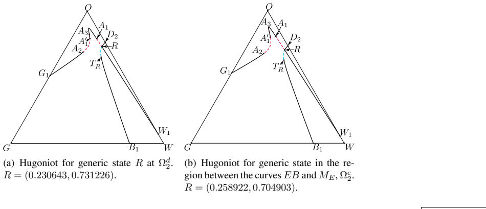
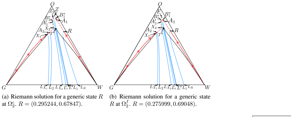
[Section 4, Claims 4.1-4.30] The central classification is presented as a series of claims whose support is largely numerical or visual. For instance, Claim 4.1 and subsequent claims describe the complete backward fast wave curve W_f(R) by referring to figures and rely on statements such as 'We verify numerically that ... satisfy the viscous profile admissibility criterion.' The orderings of the intersection points L_1, L_R, L_*, L_3, L_2 along the edge G-W, which determine the left-state intervals in each claim, are asserted from the figures rather than proved. Combined with the explicit statement that uniqueness is not established, the phrase 'we classify all Riemann solution problems' overstates what is demonstrated: the paper provides a conjectured classification based on numerical evidence and geometric inspection. The authors should either supply proofs for the structural properties of the wave curves and the left-state orderings, or clearly rephrase the claims as a numerically supported classification and remove the word 'all' from the main claims.

minor comments (5)

[Claim 4.5] The claim states that R lies in subregion Θ^b_1, but the surrounding text and Figure 13 indicate that the intended subregion is Θ^e_1; this should be corrected.
[Figure 25 caption] The caption refers to 'the ODE system (4.3)', but the relevant system is Eq. (9); the reference should be updated.
[Section 5, Cases 1 and 3] There are typos such as 'ans-rarefaction' instead of 'an s-rarefaction' and 'The numerical simulation match' instead of 'The numerical simulation matches'; these should be corrected.
[Section 3.1, Eq. (9) and surrounding text] The definition of ξ contains an unbalanced parenthesis: 'ξ=x−σt)/ε' should be 'ξ=(x−σt)/ε'.
[Claim 4.1] The sentence 'Refer to Fig. 6W f (R) comprises states M...' is missing a period after 'Fig. 6'; it should read 'Refer to Fig. 6. W_f(R) comprises states M...'.

Circularity Check

0 steps flagged · score 2.0 of 10

No significant circularity: the classification is conditional on an explicitly stated D=I viscous-profile criterion and is checked against independent numerical simulations; self-citations to prior work are not load-bearing.

full rationale

The paper's derivation chain is self-contained and non-circular. The Riemann solutions are constructed by the wave curve method (Section 3.2) from rarefaction curves, Hugoniot loci (Eq. (7)), and admissible shocks selected by the viscous profile criterion of Eq. (9). The only parametric simplification is D(S)=I, stated explicitly in Section 3.1 ('we assume D(S) to be the identity matrix and numerically verify the admissibility of shocks') and in Remark 3.1; this restricts the model but does not make any output equal to an input. The regions Theta, Omega, Gamma and their subregions are defined by geometric loci (inflection, hysteresis, double contact, mixed contact, tangential extension), not by the claimed Riemann solution structure, so the classification is not definitionally circular. No parameter is fitted to data and no 'prediction' is a renamed fit. The citations to the authors' prior work [1,2,3,4] supply published foundational facts (real characteristic speeds, explicit Hugoniot loci on invariant lines, earlier solution classes in region Lambda); these are parameter-free results with stated assumptions that do not include the present classification, so they constitute real evidence rather than a self-citation chain. The paper explicitly disclaims uniqueness ('we do not establish the uniqueness of the Riemann solution'), so no uniqueness theorem is imported to force the answer. Section 5 validates representative solutions against an independent finite-difference scheme, providing an external check. The D=I simplification is a physical limitation (the admissible shock set may change for non-identity capillary pressure), but that is a correctness or scope issue, not circularity.

Assumptions & free parameters 0 free parameters · 5 assumptions · 0 invented entities

The central claim rests on the quadratic Corey model, the identity viscosity matrix for admissibility, prior theorems from the authors' group, and an extra viscosity-regime restriction not stated in the abstract. There are no free parameters fitted to data.

assumptions (5)

domain assumption The quadratic relative permeability (Corey) model (2) accurately represents three-phase flow in the regimes of interest.
The entire analysis is performed for this specific flux function, which the paper states allows explicit calculations; results may not carry over to other Corey exponents.
domain assumption Shock admissibility is determined by the viscous profile criterion with identity viscosity matrix D(S) = I.
Section 3.1 states: 'we assume D(S) to be the identity matrix and numerically verify the admissibility of shocks.' This simplification could alter admissible shocks if the true D is different.
domain assumption The characteristic speeds and integral curve properties established in [4] hold.
The paper relies on these prior theorems for the wave curve construction; they are not re-derived here.
ad hoc to paper The double contact locus has only one branch in the saturation triangle.
Section 2: 'The viscosities are further restricted so that the double contact locus possesses only one branch in the saturation triangle.' This is an extra restriction beyond inequalities (5), conflicting with the abstract's claim of validity for all (5).
domain assumption The umbilic point lies in regions ABO or A'B'O, corresponding to Case II of the Schaeffer-Shearer classification.
Section 1 and 2 restrict attention to this regime; it is a modeling choice for heavy oil viscosities.

how reviews work

0 comments

Cite this review

Pith. "Pith review of Displacement of three-phase flow for Heavy Oil: Riemann Solutions." pith.science (2026). https://pith.science/paper/V3RULBKH

@misc{pith2026250609077,
  author       = {Pith},
  title        = {Pith review of: Displacement of three-phase flow for Heavy Oil: Riemann Solutions},
  year         = {2026},
  howpublished = {\url{https://pith.science/paper/V3RULBKH}},
  note         = {Machine review of arXiv:2506.09077}
}

abstract

This work presents the Riemann solution for three-phase flow in porous media under the condition that oil viscosity exceeds that of water and gas. We classify all Riemann solution problems for scenarios where the left states $L$ lie along the edge $G$-$W$, and the right states $R$ span nearly the entire saturation triangle, excluding small regions near the boundaries $G$-$O$ and $W$-$O$. We use the wave curve method to determine the Riemann solution for initial and injection data within the above-mentioned class. This study extends previous analytical solutions, which were limited to right states near the corner $O$ or within the quadrilateral $O$-$E$-$\mathcal{U}$-$D$. Notably, this classification remains valid for all viscosity variations satisfying the inequalities \eqref{eq:classical}, corresponding to viscosity regimes where the umbilic point is close to the vertex $O$. We verify the $L^1_{loc}$-stability of the Riemann solution with respect to variations in the data. While we do not establish the uniqueness of the Riemann solution, extensive numerical experiments confirm its validity. Our findings provide a comprehensive framework for understanding three-phase flow dynamics in porous media under a wide range of conditions.

Figures

Figures reproduced from arXiv: 2506.09077 by the authors.

**Figure 2.** Secondary bifurcation loci G - D, W - E, O - B. Segments B - U, D - U, and E - U are invariant under the slow-characteristic vector field. Segments G - U, W - U, and O - U are invariant under the fast-characteristic vector field. fig:SecBifurc (a) Slow-family integral curves. (b) Fast-family integral curves [PITH_FULL_IMAGE:figures/full_fig_p008_2.png] view at source ↗

**Figure 3.** Integral curves and inflection loci within the saturation triangle [PITH_FULL_IMAGE:figures/full_fig_p008_3.png] view at source ↗

Figures from the paper (41 more)

**Figure 4.** Figure 4: (a) State Ih is the “summit” of Is in [PITH_FULL_IMAGE:figures/full_fig_p009_4.png]

**Figure 5.** Figure 5: The relevant parts of some bifurcation loci. (a) [PITH_FULL_IMAGE:figures/full_fig_p013_5.png]

**Figure 6.** Figure 6: Subdivision of ∆ into R-regions Λ, Θ, Ω, and Γ. fig:RRegions Completed segment C ′ 3 -E on the edge G - O of the saturation triangle. Region Ω, see Figs. 6 and 7(b), is bounded by the invariant segment D - U; the segment U-P of the fast inflection locus and the segment…

**Figure 7.** Figure 7: Subdivisions of regions Θ, Ω and Γ. fig:RegioesThetas 15 [PITH_FULL_IMAGE:figures/full_fig_p015_7.png]

**Figure 8.** Figure 8: R-regions Θ1, Θ2, Θ3 in [PITH_FULL_IMAGE:figures/full_fig_p016_8.png]

**Figure 9.** Figure 9: Backward Hugoniot curves for R in subregions of Θ1, Figs. 7(a) and 8(a). Admissible slow-family shock segments: (R, T R s ] in (a) and (c); (R, TR] in (b) and (d). Admissible fastfamily shock segments: [A1, R) and [A2, A3]. We have: σ(A1; R) = λf(A1), σ(A2; R) = λf(A2…

**Figure 10.** Figure 10: Backward fast-family wave curve of R for Θ1. (a) R = (0.0402518, 0.913397) in subregion Θa 1 ∪ Θb 1 in [PITH_FULL_IMAGE:figures/full_fig_p020_10.png]

**Figure 11.** Figure 11: Riemann solution for R in the subregion Θa 1 ∪ Θc 1 with L along the edge G - W. The segments (G, T R o ]ext and (W, T R o ]ext are backward slow-extensions of segments (G, A∗ 1 ] and (W, A∗ 2 ] on Wf (R), with σ(M′ ; M) = λs(M′ ), for all M′ in [G, TR]ext ∪ [W, TR]ex…

**Figure 12.** Figure 12: Riemann solutions for R in the subregion of Θ1 with L along the edge G - W. fig:RSRinR10CandD (v) if L ∈ (L3, L∗ ), then the Riemann solution is L p Rs −→ T1 ′Ss −→ M′ 1 p Sf ′ −→ M1 Rf −→ R, where T1 ∈ (W, T∗ )ext, M′ 1 ∈ (B∗ 2 , A3) and M1 ∈ (B∗ 1 , R). rem:L*B* Rem…

**Figure 13.** Figure 13: Riemann solutions for R in the subregion Θe 1 in [PITH_FULL_IMAGE:figures/full_fig_p024_13.png]

**Figure 14.** Figure 14: Hugoniot curve for R in the subregion of Θ2. We have σ(A1; R) = λf(A1), σ(TR; R) = λs(TR). The segments (R, A1] and (R, TR] are admissible. fig:Hugoniot_R3 locus If ; and segment IE-C3 of the edge G - O. As shown in [PITH_FULL_IMAGE:figures/full_fig_p025_14.png]

**Figure 15.** Figure 15: R in subregion of Θ2 bounded by Θa 2 of [PITH_FULL_IMAGE:figures/full_fig_p028_15.png]

**Figure 16.** Figure 16: Wave Curves fig:Wave_Curves_Theta_2_b_Theta_2_c (a) Riemann solution for R in subregion Θb 2 (b) Riemann solution for R in subregion Θc 2 [PITH_FULL_IMAGE:figures/full_fig_p029_16.png]

**Figure 17.** Figure 17: Riemann solution for R in Θ2 with R below the invariant segment C2 - I f 2 of [PITH_FULL_IMAGE:figures/full_fig_p029_17.png]

**Figure 18.** Figure 18: Backward Hugoniot curve based on R in subregion Θa 3 . The detached branch [D1, W1] in (b) is not admissible according to the viscous profile criterion. We have: σ(A1; R) = λf(A1), σ(A4; R) = λf(A4), σ(TR; R) = λs(TR) fig:BFWC-R4_Above Refer to Figs. 18, 19, and 20. A…

**Figure 19.** Figure 19: Backward Hugoniot curve based on R in subregion Θb 3 . The detached branch [D1, W1] in (b) is not admissible according to the viscous profile criterion. We have: σ(A1; R) = λf(A1), σ(A4; R) = λf(A4), σ(TR; R) = λs(TR). fig:BFWC-R4_belowB (a) R = (0.109168, 0.715865). …

**Figure 20.** Figure 20: Backward Hugoniot curve for R in subregion Θc 3 . We have: σ(A1; R) = λf(A1) and σ(TR; R) = λs(TR). figBlowFWC-R4_beC 31 [PITH_FULL_IMAGE:figures/full_fig_p031_20.png]

**Figure 21.** Figure 21: (a) Admissible Wf (R); (b) Riemann solution for R ∈ Θa 3 . The curve [G, T∗ ]ext ∪ [T ∗ , W]ext is an extension of the Wf (R) segment [G, B∗ 1 ] ∪ [B∗ 2 , W] such that σ(M′ , M) = λs(M′ ) for all M′ ∈ [G, T∗ ]ext ∪ [T ∗ , W]ext and M ∈ [G, B∗ 1 ] ∪ [B∗ 2 , W]. For thi…

**Figure 22.** Figure 22: (a) Wf (R); (b) Riemann solution for R ∈ Θb 3 . The curve [G, T∗ ]ext ∪ [T ∗ , W]ext is an extension of the Wf (R) segment [G, B∗ 1 ] ∪ [B∗ 2 , W] such that σ(M′ , M) = λs(M′ ) for all M′ ∈ [G, T∗ ]ext ∪ [T ∗ , W]ext and M ∈ [G, B∗ 1 ] ∪ [B∗ 2 , W]. For this case, we …

**Figure 23.** Figure 23: Admissible Wf (R) and Riemann solution for R ∈ Θ3 in subregion bounded by Θc 3 . Curve [G, T∗ 1 ]ext ∪[T ∗ 1 , W]ext is an extension of the Wf (R) segment [G, B∗ 1 ]∪[B∗ 2 , W] such that σ(M′ , M) = λs(M′ ), for all (M′ , M) ∈ [G, T∗ 1 ]ext ∪ [T ∗ 1 , W]ext × [G, B∗ 1…

**Figure 24.** Figure 24: Zoom of the R-regions Ω1 and Ω2 in [PITH_FULL_IMAGE:figures/full_fig_p036_24.png]

**Figure 25.** Figure 25: Some orbits of the ODE system (4.3) for M in the detached segment [PITH_FULL_IMAGE:figures/full_fig_p037_25.png]

**Figure 26.** Figure 26: Hugoniot for generic states R in Ω2 fig:Hugoniot_Omega_2A the states in Wf (R) with σ(A1; R) = λf(A1), λf (A1) = σ(A1; R) = σ(A′ 1 ; A1) = σ(A′ 1 ; R), λs(T ∗ ) = σ(T ∗ ; B∗ 1 ) = λf(B∗ 1 ) = σ(B∗ 2 ; B∗ 1 ) = σ(T ∗ ; B∗ 2 ), with T ∗ ∈ H(B∗ 1 ). Let L2, L ′ 1 , L ∗ ,…

**Figure 27.** Figure 27: Hugoniot for generic states R in Ω2. fig:Hugoniot_Omega_2B (vii) if L = W, the Riemann solution is W p Rf −→ R. rem:L*B*4 Remark 4.7. If L = L ∗ , see [PITH_FULL_IMAGE:figures/full_fig_p039_27.png]

**Figure 28.** Figure 28: Hugoniot for generic states R in Ω2. fig:Hugoniot_Omega_2C cla:RSolution-Omega_2bU2e Claim 4.16. Refer to [PITH_FULL_IMAGE:figures/full_fig_p040_28.png]

**Figure 29.** Figure 29: Hugoniot for generic states R in Ω2. fig:Hugoniot_Omega_2D (vii) if L ∈ (L ′ 1 , L∗ ), the Riemann solution is L p Rs −→ T1 ′Ss −→ M′ 1 p Sf ′ −−→ M1 Rf −→ A1 ′Sf −−→ R, where T1 ∈ (X2, T∗ ]ext, M′ 1 ∈ (A′ 1 , B∗ 2 ) and M1 ∈ (B∗ 1 , A1); (viii) if L ∈ (L ∗ , L1), the…

**Figure 30.** Figure 30: Wave Curve for a generic states R in Ω2 fig:Wave_Curve_2A shock rule guarantees they represent the same solution in xt-space. In other words, the solution consists of a single wave group. We now consider R in region Ω h 2 . The changes in the Riemann solutions when R …

**Figure 31.** Figure 31: Riemann solution for a generic states R in Ω2. fig:Wave_Curve_2B (i) if L = G, the Riemann solution is G p Rf −→ A2 ′Sf −−→ R; (ii) if L ∈ (G, LX1 ), the Riemann solution is L p Rs −→ T1 ′Ss −→ M1 p Rf −→ A2 ′Sf −−→ R, where T1 ∈ (G, X1)ext and M1 ∈ (G, X1); (iii) if …

**Figure 32.** Figure 32: Riemann solution for a generic states R in Ω2 fig:Wave_Curve_2C rem:L*B*6 Remark 4.10. If L = L ∗ , see [PITH_FULL_IMAGE:figures/full_fig_p044_32.png]

**Figure 33.** Figure 33: Wave Curve for a generic states R in Ω2 fig:Wave_Curve_2D Typical backward fast wave curves Wf (R) for R in Γ1 and Γ2 far from edge G - W are shown in Figs. 40 and 41, where it is also shown geometric representations of Riemann solutions. Such wave curves consist of …

**Figure 34.** Figure 34: Riemann solution for a generic states R in Ω2 fig:Wave_Curve_2E σ(A1; R) = λf(A1). Let L1 and LR be the intersection points of the backward slow wave curves of A1 and R with the edge G - W. Then, (i) if L = G, the Riemann solution is G p Rf −→ A1 ′Sf −−→ R ; (ii) if L…

**Figure 35.** Figure 35: Riemann solution for a generic states R in Ω2 fig:Wave_Curve_2F (i) if L = G, the Riemann solution is G p Rf −→ A1 ′Sf −−→ R; (ii) if L ∈ (G, L1) the Riemann solution is L p Rs −→ T1 ′Ss −→ M1 p Rf −→ A1 ′Sf −−→ R, where T1 ∈ (G, X1)ext and M1 ∈ (G, A1); (iii) if L ∈ …

**Figure 36.** Figure 36: Wave Curve for a generic states R in Ω2 fig:Wave_Curve_2G Let L1, LX1 , LX2 and LR be the intersection points of the backward slow wave curves of A1, X1, X2 and R with the edge G - W. Then, (i) if L = G, the Riemann solution is G p Rf −→ A1 ′Sf −−→ R ; (ii) if L ∈ (G,…

**Figure 37.** Figure 37: Riemann solution for a generic state R in Ω2. fig:Wave_Curve_2H cla:RSolution-Gamma_1d-new Claim 4.23. Refer to [PITH_FULL_IMAGE:figures/full_fig_p049_37.png]

**Figure 38.** Figure 38: Zoom of the R-regions Γ1 and Γ2 in [PITH_FULL_IMAGE:figures/full_fig_p050_38.png]

**Figure 39.** Figure 39: Hugoniot curves for states R in Γ1 and Γ2, far from edge G - W. fig:Hugoniot_Gamma_regions 51 [PITH_FULL_IMAGE:figures/full_fig_p051_39.png]

**Figure 40.** Figure 40: Wave curves Wf (R) and Riemann solutions for states R in Γ1. fig:Solution_Riemann_P_Gamma_1 52 [PITH_FULL_IMAGE:figures/full_fig_p052_40.png]

**Figure 41.** Figure 41: Wave curves Wf (R) and Riemann solutions for states R in Γ2. fig:Solution_Riemann_P_Gamma_2 55 [PITH_FULL_IMAGE:figures/full_fig_p055_41.png]

**Figure 42.** Figure 42: (a) illustrates the analytical solution for the Riemann problem with initial states L ∈ (G, L2) and R ∈ Ω a 1 . The composition path ( [PITH_FULL_IMAGE:figures/full_fig_p059_42.png]

**Figure 43.** Figure 43: Analytical solution for R ∈ Ω b 1 and L ∈ (L ∗ , L3). (a) The composition path in the saturation triangle that consists of L p Rs −→ T ′Ss −→ M′ p Sf ′ −−→ M Rf −→ R. The gray curve segments are the parts of the slow and fast wave curves that are not involved in the s…

**Figure 44.** Figure 44: Analytical solution for R ∈ Ω a 2 and L ∈ [L1, LR). (a) The composition path in the saturation triangle, consisting of an s-rarefaction from L to T, follows an s-shock from T to M, and an f-shock from M to R. The gray curve segments are the parts of the slow and fast …

Discussion (0). Sign in to comment.

Reference graph

Works this paper leans on

32 extracted references · 31 canonical work pages

[1]

Andrade, A

P. Andrade, A. de Souza, F. Furtado, and D. Marchesin. Oil displacement by water and gas in a porous medium: the Riemann problem . Bull. Braz. Math. Soc. (N.S.), 47 0 (1): 0 1--14, 2016

work page 2016
[2]

Andrade, A

P. Andrade, A. de Souza, F. Furtado, and D. Marchesin. Three-phase fluid displacement in a porous medium . Journal of Hyperbolic Differential Equations, 15 0 (4): 0 731--753, 2018

work page 2018
[3]

Azevedo, A

A. Azevedo, A. de Souza, F. Furtado, D. Marchesin, and B. Plohr. The solution by the wave curve method of three-phase flow in virgin reservoirs . Transport in Porous Media, 83 0 (1): 0 99--125, 2010

work page 2010
[4]

Azevedo, A

A. Azevedo, A. de Souza, F. Furtado, and D. Marchesin. Uniqueness of the Riemann solution for three-phase flow in a porous medium . SIAM J. Appl. Math., 74 0 (6): 0 1967--1997, 2014

work page 1967
[5]

A. V. Azevedo, D. Marchesin, B. Plohr, and K. Zumbrun. Capillary instability in models for three-phase flow. Zeitschrift f \"u r angewandte Mathematik und Physik ZAMP , 53: 0 713--746, 2002

work page 2002
[6]

A critical review on parameters affecting the feasibility of underground hydrogen storage

Chiradip Bagchi, Samarth D Patwardhan, Stefan Iglauer, Hisham Ben Mahmud, and Muhammad Fazil Jaffar Ali. A critical review on parameters affecting the feasibility of underground hydrogen storage. ACS Omega, 2025

work page 2025
[7]

Analytical solution for one-dimensional three-phase incompressible flow in porous media for concave relative permeability curves

Wagner Q Barros, Adolfo P Pires, and Alvaro MM Peres. Analytical solution for one-dimensional three-phase incompressible flow in porous media for concave relative permeability curves. International Journal of Non-Linear Mechanics, 137: 0 103792, 2021

work page 2021
[8]

Safety of hydrogen storage technologies

Emma Davies, Andrea Ehrmann, and Eva Schwenzfeier-Hellkamp. Safety of hydrogen storage technologies. Processes, 12 0 (10): 0 2182, 2024

work page 2024

Show all 32 references

[9]

de Souza

A. de Souza. Stability of singular fundamental solutions under perturbations for flow in porous media . Mat. Apl. Comput., 11 0 (2): 0 43, 1992

1992
[10]

ELI , I nteractive G raphical R iemann P roblem S olver

ELI. ELI , I nteractive G raphical R iemann P roblem S olver. https://eli.fluid.impa.br/, pages A ccessed : 2025--06--08, 2025

2025
[11]

Lozano L. F. Diffusive effects in Riemann solutions for the three phase flow in porous media, D.Sc. thesis . PhD thesis, Instituto de Matem \' a tica Pura e Aplicada (IMPA), Rio de Janeiro, Brazil , 2018

2018
[12]

Isaacson, D

E. Isaacson, D. Marchesin, and B. Plohr. Transitional waves for conservation laws . SIAM J. Math. Anal., 21 0 (4): 0 837--866, 1990

1990
[13]

Isaacson, D

E. Isaacson, D. Marchesin, B. Plohr, and B. Temple. Multiphase flow models with singular Riemann problems . Comput. Appl. Math., 11 0 (2): 0 147--166, 1992

1992
[14]

Data-driven prediction of in situ co2 foam strength for enhanced oil recovery and carbon sequestration

Javad Iskandarov, George S Fanourgakis, Shehzad Ahmed, Waleed Alameri, George E Froudakis, and Georgios N Karanikolos. Data-driven prediction of in situ co2 foam strength for enhanced oil recovery and carbon sequestration. RSC advances, 12 0 (55): 0 35703--35711, 2022

2022
[15]

Analytical solution to the riemann problem of three-phase flow in porous media

Ruben Juanes and Tadeusz W Patzek. Analytical solution to the riemann problem of three-phase flow in porous media. Transport in Porous Media, 55: 0 47--70, 2004

2004
[16]

Mathematics and numerics for balance partial differential-algebraic equations (pdaes)

Wanderson Lambert, Amaury Alvarez, Ismael Ledoino, Duilio Tadeu, Dan Marchesin, and Johannes Bruining. Mathematics and numerics for balance partial differential-algebraic equations (pdaes). J. Sci. Comput., 84 0 (2): 0 29, 2020. doi:10.1007/s10915-020-01279-w

2020 doi
[17]

P. Lax. Hyperbolic systems of conservation laws II . Comm. Pure Appl. Math., X, 1952

1952
[18]

T. P. Liu. The Riemann problem for general 2x2 conservations laws . Trans. Amer. Math. Soc., 199: 0 89--112, 1974

1974
[19]

T. P. Liu. The Riemann problem for general systems of conservations laws . J. Differential Equations, 18: 0 218--234, 1975

1975
[20]

Analytical investigation of the three-phase foam flow in porous media

L Lozano, G Chapiro, and D Marchesin. Analytical investigation of the three-phase foam flow in porous media. In ECMOR 2024, volume 2024, pages 1--9. European Association of Geoscientists & Engineers, 2024 a

2024
[21]

Lozano, I

L. Lozano, I. Ledoino, B. J . Plohr, and D. Marchesin. Structure of undercompressive shock waves in three-phase flow in porous media, 2024 b . URL https://arxiv.org/abs/2412.04439

2024 arXiv
[22]

Matos, A

V. Matos, A. Azevedo, J. Mota, and D. Marchesin. Bifurcation under parameter change of Riemann solutions for nonstrictly hyperbolic systems . Z. Angew. Math. Phys., 66 0 (4): 0 1413--1452, 2015

2015
[23]

Matos, J

V. Matos, J. D. Silva, and D. Marchesin. Loss of hyperbolicity changes the number of wave groups in Riemann problems . Bulletin of the Brazilian Mathematical Society, 47 0 (2): 0 545--559, 2016

2016
[24]

Solution construction to a class of R iemann problems of multiphase flow in porous media

Mehran Mehrabi, Kamy Sepehrnoori, and Mojdeh Delshad. Solution construction to a class of R iemann problems of multiphase flow in porous media. Transport in porous media, 132: 0 241--266, 2020

2020
[25]

Core flooding experimental study on enhanced oil recovery of heavy oil reservoirs with high water cut by sub-and supercritical water

Yan Miao, Qiuyang Zhao, Zujie Huang, Keyu Zhao, Hao Zhao, Liejin Guo, and Yechun Wang. Core flooding experimental study on enhanced oil recovery of heavy oil reservoirs with high water cut by sub-and supercritical water. Geoenergy Science and Engineering, 242: 0 213208, 2024

2024
[26]

Approximate analytical solutions for 1-d immiscible water alternated gas

Adolfo P Pires, Wagner Q Barros, and Alvaro MM Peres. Approximate analytical solutions for 1-d immiscible water alternated gas. Transport in Porous Media, 151 0 (1): 0 171--191, 2024

2024
[27]

The influence of capillary pressure on the phase equilibrium of the co2--water system: Application to carbon sequestration combined with geothermal energy

Hamidreza Salimi, Karl-Heinz Wolf, and Johannes Bruining. The influence of capillary pressure on the phase equilibrium of the co2--water system: Application to carbon sequestration combined with geothermal energy. International Journal of Greenhouse Gas Control, 11: 0 S47--S66, 2012

2012
[28]

The classification of 2 2 systems of non-strictly hyperbolic conservation laws, with application to oil recovery

David G Schaeffer and Michael Shearer. The classification of 2 2 systems of non-strictly hyperbolic conservation laws, with application to oil recovery. Communications on pure and applied mathematics, 40 0 (2): 0 141--178, 1987

1987
[29]

Riemann solutions without an intermediate constant state for a system of two conservation laws

Julio Daniel Silva and Dan Marchesin. Riemann solutions without an intermediate constant state for a system of two conservation laws. Journal of Differential Equations, 256 0 (4): 0 1295--1316, 2014

2014
[30]

Foam-oil displacements in porous media: Insights from three-phase fractional-flow theory

Jinyu Tang, Pablo Castaneda, Dan Marchesin, and William R Rossen. Foam-oil displacements in porous media: Insights from three-phase fractional-flow theory. In Abu Dhabi International Petroleum Exhibition and Conference, page D042S195R003. SPE, 2022

2022
[31]

Wendroff

B. Wendroff. The Riemann problem for materials with Non Convex Equations of state: I Isentropic flow; II General flow . J. Math. Anal Appl., 38 0 (2--3): 0 454 -- 466; 640 -- 658, 1972

1972
[32]

Enhanced heavy oil recovery by immiscible WAG injection

YP Zhang, S Sayegh, and S Huang. Enhanced heavy oil recovery by immiscible WAG injection. In PETSOC Canadian International Petroleum Conference, pages PETSOC--2006. PETSOC, 2006

2006

Pith tools

Reviewed August 7, 2026 · model on record in the stance chip above.

[1] [1]

Andrade, A

P. Andrade, A. de Souza, F. Furtado, and D. Marchesin. Oil displacement by water and gas in a porous medium: the Riemann problem . Bull. Braz. Math. Soc. (N.S.), 47 0 (1): 0 1--14, 2016

work page 2016

[2] [2]

Andrade, A

P. Andrade, A. de Souza, F. Furtado, and D. Marchesin. Three-phase fluid displacement in a porous medium . Journal of Hyperbolic Differential Equations, 15 0 (4): 0 731--753, 2018

work page 2018

[3] [3]

Azevedo, A

A. Azevedo, A. de Souza, F. Furtado, D. Marchesin, and B. Plohr. The solution by the wave curve method of three-phase flow in virgin reservoirs . Transport in Porous Media, 83 0 (1): 0 99--125, 2010

work page 2010

[4] [4]

Azevedo, A

A. Azevedo, A. de Souza, F. Furtado, and D. Marchesin. Uniqueness of the Riemann solution for three-phase flow in a porous medium . SIAM J. Appl. Math., 74 0 (6): 0 1967--1997, 2014

work page 1967

[5] [5]

A. V. Azevedo, D. Marchesin, B. Plohr, and K. Zumbrun. Capillary instability in models for three-phase flow. Zeitschrift f \"u r angewandte Mathematik und Physik ZAMP , 53: 0 713--746, 2002

work page 2002

[6] [6]

A critical review on parameters affecting the feasibility of underground hydrogen storage

Chiradip Bagchi, Samarth D Patwardhan, Stefan Iglauer, Hisham Ben Mahmud, and Muhammad Fazil Jaffar Ali. A critical review on parameters affecting the feasibility of underground hydrogen storage. ACS Omega, 2025

work page 2025

[7] [7]

Analytical solution for one-dimensional three-phase incompressible flow in porous media for concave relative permeability curves

Wagner Q Barros, Adolfo P Pires, and Alvaro MM Peres. Analytical solution for one-dimensional three-phase incompressible flow in porous media for concave relative permeability curves. International Journal of Non-Linear Mechanics, 137: 0 103792, 2021

work page 2021

[8] [8]

Safety of hydrogen storage technologies

Emma Davies, Andrea Ehrmann, and Eva Schwenzfeier-Hellkamp. Safety of hydrogen storage technologies. Processes, 12 0 (10): 0 2182, 2024

work page 2024