REVIEW 4 major objections 5 minor 60 references
The ATLAS Virtual Research Assistant
T0 review · 4 major / 5 minor · reviewed 2026-08-07 · deepseek-v4-flash
Pith's one-line read The ATLAS Virtual Research Assistant ranks alerts by real and extragalactic scores and, in production, cut eyeballing workload by 85% while losing under 0.08% of follow-up opportunities.
desk verdict A genuinely useful operations paper: the VRA convincingly cuts eyeballing workload by ~85% while keeping recovery of extragalactic transients high; the headline 'loss' metric is a lower bound, not the whole story. read the letter →
The pith
A machine-rendered reading of the paper's core claim, the machinery that carries it, and where it could break.
The reading
What carries the argument
The load-bearing object is the two-dimensional 'score space' with axes $p_{\rm real}$ and $p_{\rm gal}$, produced by four histogram-based gradient-boosted decision tree classifiers (day-1 and day-N versions of real/bogus and galactic/extragalactic). Alerts are ranked by the VRA score, a normalized geometric distance to the ideal extragalactic point, $$\mathrm{VRAscore}=10\times\frac{\sqrt{$f^{2}$+1}-\sqrt{(1-p_{\rm real})^2+(f\,p_{\rm gal})^2}}{\sqrt{$f^{2}$+1}},$$ with a galactic-axis scaling factor $f=0.5$ that weights the Real axis twice as heavily as the Galactic axis. The evaluation metric is recall at rank $K$ (R@K), with an area-under-curve variant AuRaK benchmarked against the pre-VRA CNN ordering; the auto-garbaging policies apply day-dependent VRA-score thresholds, discarding alerts below 1 on day 1, below 2 on the second visit, and below 3 on later visits.
What would settle it
Re-eyeball every alert auto-garbaged during the production window 2025-04-04 to 2025-06-10, using forced photometry or independent classification, and count how many are genuine extragalactic transients; if that fraction exceeds the paper's reported 0.079% loss of extragalactic events, the central claim would be refuted.
Extended reading notes
Core claim
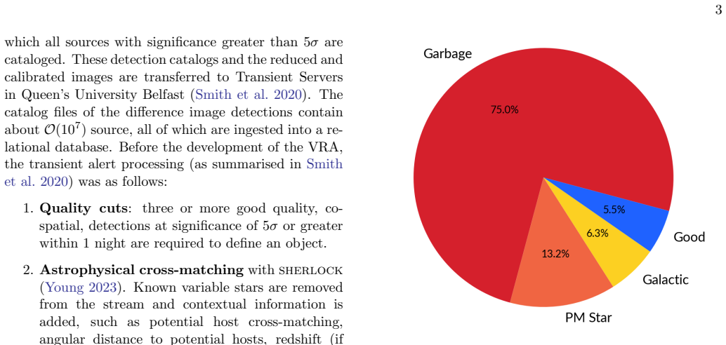
The central claim is that alert triage in a messy transient stream can be reduced to two binary questions—'Is it real?' and 'Is it galactic?'—answered by gradient-boosted decision trees trained on human eyeball labels. Each alert gets a Real score and a Galactic score; these are combined into a single 0–10 VRA score defined as a normalized distance to the (real=1, galactic=0) corner of score space, with TNS cross-matches promoted to rank 10 and new light-curve visits updating the scores through separate day-1 and day-N models. On the validation set, ordering by the day-1 models recovers 95% (99%) of the 'Good' extragalactic alerts in the top 15% (25%) of the list, compared with 35% (60%) for the previous CNN real-bogus ordering, and the day-N models reach 95% recall in the top 5% of the list. In production from April to June 2025, the auto-garbaging policies removed 85% of 16,938 alerts from the eyeball list, and the authors place the missed follow-up opportunity at 0.006% of all alerts and 0.079% of extragalactic events.
Load-bearing premise
The human labels that train and validate the models are treated as accurate ground truth, even though the paper notes PM/Garbage confusion, duplicates and AGNs in the Attic, and only partial re-eyeballing; if label errors concentrate in the extragalactic class, the reported recall and loss figures could be optimistic.
Editorial extensions
If this is right
- In production, each day's eyeball list shrinks to roughly one-sixth of its pre-VRA size because 85% of alerts are auto-garbaged, and the remaining list is ranked so human scanners see the most promising extragalactic candidates first.
- The day-N models use new detection and non-detection information from later visits, so an alert's rank improves as its light curve grows; validation shows 95% recall of Good objects in the top 5% of the ordered list.
- The same scores drive automated follow-up triggers on the Lesedi telescope, meaning a single learned score stream can both rank for humans and activate robotic observations.
- The R@K benchmark gives other surveys a direct test: a replacement triage model must beat the AuRaK of the existing ordering before it is worth deploying.
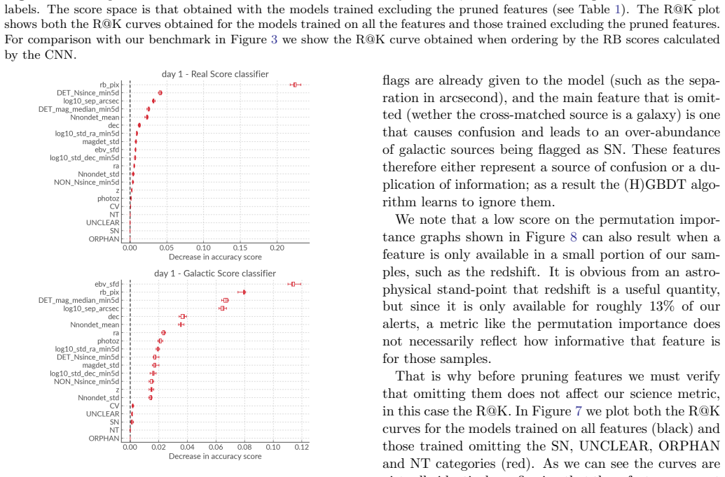
- Feature-based classifiers trained on a few thousand examples can match or exceed neural-network ordering in this setting, offering interpretability and a route to inject domain knowledge.
Reading between the lines
- The 85% auto-garbage fraction was measured during a window that included an anomalous week of image trailing; steady-state workload reduction may be closer to the 80.2% predicted from validation than to 85%.
- The reported loss rate depends on TNS cross-matching to catch misses, so genuine losses that neither VRA nor TNS flags would go uncounted; a forced-photometry audit of auto-garbaged alerts would test this.
- Transferring this design to LSST or ZTF will require retraining on each survey's artifacts and cadence, since features like extinction and RA/Dec encode ATLAS-specific tiling and moon-phase effects, but the score-space ranking recipe is survey-agnostic.
- Extending the score space with the deprioritized 'fast' axis, or adding forced-photometry features on day N, is a natural next step that the authors flag as future work.
Editorial analysis
A structured set of objections, weighed in public.
Referee Report
Summary. The paper presents the ATLAS Virtual Research Assistant (VRA), a production system that ranks transient alerts using two Histogram-Based Gradient Boosted Decision Tree classifiers ('Real' and 'Galactic'), with separate day-1 and day-N models that incorporate new light-curve information. Alerts are ranked by a geometric VRA score (Eq. 2), and eyeballing/auto-garbaging policies select which alerts humans inspect. The authors benchmark their ranking with Recall at rank K and AuRaK against the pre-existing Real/Bogus CNN ordering, evaluate policies on a validation set, and report in-production statistics from 2025-04-04 to 2025-06-10, claiming an 85% reduction in eyeballing workload with a <0.08% loss of follow-up opportunity. The system also automatically triggers follow-up observations with the Lesedi telescope.
Significance. If the central claims hold, the VRA is a practical, interpretable, and low-cost automation of transient alert triage that is highly relevant to current and future surveys (e.g., LSST). The paper's strengths include a clear benchmark against the pre-VRA RB-score strategy, explicit release of code and training data (Zenodo), transparent reporting of in-production monitoring including 'potential misses', and a design that uses only a few thousand training samples. These are substantial contributions to astroinformatics practice. The main weakness is that the headline loss metric is conditional on TNS independent discovery, and the training and policy evaluation involve a self-referential loop that the paper acknowledges only in part.
major comments (4)
- [Section 4.2 and abstract] The headline figure '<0.08% loss of follow-up opportunity' is computed by cross-matching auto-garbaged alerts to TNS (Sections 2.6 and 4.2). This metric only counts transients that were independently reported to TNS by another survey; any transient that ATLAS alone would have recovered pre-VRA but that no other facility noticed is invisible to the estimate. The paper's own monitoring text supports this concern: 164 'potential misses', 34 below threshold for 15 days, 20 real events, and 1 potentially follow-up-worthy (SN2025hkm) were found only because of the TNS cross-match. The loss rate should therefore be stated as a TNS-conditional lower bound, and the abstract and conclusion should not present it as an overall loss rate without this qualification. A random-sample manual review of auto-garbaged alerts or forced-photometry checks would provide a more complete estimate.
- [Section 5.4 and Section 4.1] The auto-garbaging thresholds (<1, <2, <3 on visits 1-3) and the eyeballing threshold (>7) were set or adjusted based on the policy evaluation of Section 4.1; Section 5.4 states that 'the values changed slightly based on the policy evaluation presented in Section 4.1'. Therefore the validation-set performance figures in Section 4.1 (e.g., 80.2% auto-garbaged, 97% of Good objects eyeballed) are in-sample estimates and cannot be read as out-of-sample predictive performance. The in-production statistics in Section 4.2 are a better external test, but the paper should explicitly separate in-sample tuning from out-of-sample validation when interpreting both sets of numbers.
- [Section 3.2 and Table 2] The training set includes 1,600 (day-1 training) and 3,571 (day-1 validation) samples labeled 'Auto-garbage' by earlier VRA versions, and this class is used as ground truth for p_real=0. Because the VRA's own outputs become training labels, any systematic errors in auto-garbaging policies are reinforced; the TNS cross-match in Section 4.2 indeed shows that real extragalactic transients can be auto-garbaged. Section 3.1 discusses human-label impurity but does not quantify the fraction of auto-garbage labels that were re-eyeballed, nor does the paper test how results change if auto-garbage samples are removed or re-weighted. This is a load-bearing circularity for the training procedure and should be addressed with a sensitivity analysis.
- [Section 4.2 vs Section 6] The abstract and Section 6 state 'no loss of follow-up opportunity' and summarize the result as an unqualified 85% workload reduction. Section 4.2 itself reports that one event (SN2025hkm) 'may have been the object of follow-up' and that the 85% figure is inflated by a hardware/weather week (7,516 alerts, 91.5% auto-garbaged in the week starting 2025-05-23). The conclusions should be qualified to match the body: an 85% reduction over a two-month window that includes a trail-rich week, and a TNS-conditional potential follow-up loss of at most one object by the paper's own accounting.
minor comments (5)
- [Section 2.6] Typo: 'prugatory sentinel' should read 'purgatory sentinel'.
- [Table 1] The description for 'NON N today' reads 'Number of detections seen today', which should be 'Number of non-detections seen today'.
- [Section 6] Spelling inconsistency: the telescope is called 'Lesedi' in Sections 2.4 and 6, but 'Lesidi' appears in Section 6 ('the 1-m Lesidi Telescope'). Please unify.
- [Section 3.2.1] Grammar: 'To illustrate this process with show in Figure 6 an example' appears to be missing a verb; consider 'To illustrate this process, we show in Figure 6 an example'.
- [Section 4.2] Minor wording: 'transients events miss-labeled' should be 'transient events mislabeled'.
Circularity Check
No fatal circularity: the workload reduction is a measured production outcome, but the loss metric is definitionally TNS-conditional, and the training/policy loop contains self-referential elements.
-
self definitional
[Section 2.6 (Monitoring) and Section 4.2 (In production performance)]
"Potential misses are defined as alerts which would have not met the VRA rank threshold but whose rank was raised to 10 by a cross-match to TNS. ... as the current potential loss rate is only 0.006% of all the alerts entering the eyeball list, and 0.079% of all the Extra Galactic events."
The loss-of-follow-up metric counts only transients that appear in TNS: a 'potential miss' is, by definition, an alert whose VRA score was low but whose rank was rescued by a TNS cross-match. Any extragalactic transient that the VRA auto-garbaged and that no other survey reported to TNS is invisible to the metric. The reported <0.08% loss is therefore not an estimate of total lost follow-up opportunity but a measure of TNS-visible loss, so the headline loss figure is partly an artifact of the definition rather than an independent measurement of all missed science.
-
fitted input called prediction
[Section 4.1.2 and Section 5.4 (Choosing the policies)]
"Based on our validation set, we can expect that over the course of a week 80.2% of the incoming alerts will be auto-garbaged, 3.7% will be left in purgatory and 16% will be sent to human scanners for eyeballing. ... In future iterations of the VRA the garbaging logic remained the same but the values changed slightly based on the policy evaluation presented in Section 4.1."
The auto-garbaging thresholds were adjusted using the Section 4.1 policy evaluation on the validation set, and then the same evaluation is quoted as an expected production outcome ('80.2% ... will be auto-garbaged'). That expectation is an in-sample consequence of thresholds fitted to that same validation set, not an out-of-sample prediction. The later production measurement of 85% is genuinely independent, so this step is a presentation weakness rather than the main result.
1 more flagged steps
-
other
[Section 3.2 (Data and Features), Table 2]
"This is the first dataset that is impacted by the VRA, which is reflected in the large fraction of data that are labelled as 'Auto-garbage'. ... Auto-garbage [preal=NaN;p_gal=0] 1,600 3,571"
A substantial part of the training and validation labels are 'Auto-garbage' outputs produced by earlier versions of the VRA itself. The classifiers are therefore being optimized, in part, to reproduce the VRA's own previous auto-garbaging decisions, creating a feedback loop in the training data. This does not force the headline result because the production loss claim is checked against TNS, but it does mean the model's agreement with 'Auto-garbage' labels is not fully independent evidence that those labels are correct.
full rationale
The central derivation is not circular in the strongest sense. The VRA classifiers are trained on human eyeballing labels (with acknowledged impurities), benchmarked against the existing CNN RB score via R@K and AuRaK, and the headline 85% workload reduction is a direct measurement on 16,938 production alerts between 2025-04-04 and 2025-06-10, not a value recovered from the training set. The TNS cross-match is an external source of ground truth, and the paper manually reviews the 34 sub-threshold potential misses, which is genuine validation effort. However, three steps contain partial self-reference or in-sample fitting. First, the loss metric counts only TNS-registered transients: a 'potential miss' is defined as an alert whose VRA score was low but whose rank was raised by TNS cross-match, so any ATLAS-only miss not reported to TNS is invisible; the <0.08% figure is therefore a bound on TNS-visible loss by construction. Second, the auto-garbaging policy thresholds were adjusted using the Section 4.1 policy evaluation, and the same evaluation is then quoted as the expected 80.2% auto-garbage fraction, so that expectation is in-sample rather than a genuine prediction; the later production number is independent. Third, a portion of the training labels are 'Auto-garbage', i.e., outputs of earlier VRA versions, so the models are partly trained to reproduce the VRA's own previous decisions; this is a feedback loop rather than a derivation, and it is mitigated by the TNS check. The self-citations to the Technical Manual and data release are for implementation details, not for load-bearing uniqueness or correctness claims. Overall the central claim has substantial independent content, so the circularity score is 4, reflecting the TNS-conditional loss definition and the in-sample policy estimate rather than a collapse of the derivation.
Assumptions & free parameters
free parameters (6)
- f (VRA score axis scaler) =
0.5
- f (galactic flag scaler) =
0.9
- galactic flag distance threshold =
<0.4
- extragalactic eyeballing threshold =
>7
- auto-garbaging thresholds =
VRA<1 day1; <2 visit2; <3 mean visit3+
- dayN cutoff =
15 days
assumptions (4)
- domain assumption Human eyeball classification is a valid ground truth for real/bogus and galactic/extragalactic status
- domain assumption TNS cross-matching of the garbage list is an adequate external audit of missed follow-up opportunities
- domain assumption The upstream cut (CNN RB score > 0.2) and other pre-VRA filtering are fixed
- ad hoc to paper The VRA score distance formula (Eq. 2) orders alerts by scientific priority
Cite this review
Pith. "Pith review of The ATLAS Virtual Research Assistant." pith.science (2026). https://pith.science/paper/RTMOVCER
@misc{pith2026250609778,
  author       = {Pith},
  title        = {Pith review of: The ATLAS Virtual Research Assistant},
  year         = {2026},
  howpublished = {\url{https://pith.science/paper/RTMOVCER}},
  note         = {Machine review of arXiv:2506.09778}
}
read the original abstract
We present the Virtual Research Assistant (VRA) of the ATLAS sky survey which performs preliminary eyeballing on our clean transient data stream. The VRA uses Histogram Based Gradient Boosted Decision Tree Classifiers trained on real data to score incoming alerts on two axes: "Real" and "Galactic". The alerts are then ranked using a geometric distance such that the most "Real" and "Extra-galactic" receive high scores; the scores are updated when new light curve data is obtained on subsequent visits. To assess the quality of the training we use the Recall at rank K, which is more informative to our science goal than general metrics such as accuracy or F1-Scores. We also establish benchmarks for our metric based on the pre-VRA eyeballing strategy, to ensure our models provide notable improvements before being added to the ATLAS pipeline. Finally, policies are defined on the ranked list to select the most promising alerts for humans to eyeball and to automatically remove the bogus alerts. In production the VRA method has resulted in a reduction in eyeballing workload by 85% with a loss of follow-up opportunity <0.08%. It also allows us to automatically trigger follow-up observations with the Lesedi telescope, paving the way to automated methods that will be required in the era of LSST. inally, this is a demonstration that feature-based methods remain extremely relevant in our field, being trainable on only a few thousand samples and highly interpretable; they also offer a direct way to inject expertise into models through feature engineering
Figures


Figures from the paper (21 more)







Reference graph
Works this paper leans on
-
[1]
Alwosheel, A., van Cranenburgh, S., & Chorus, C. G. 2018, Journal of Choice Modelling, 28, 167, doi: https://doi.org/10.1016/j.jocm.2018.07.002
-
[2]
Bellm, E. C., Kulkarni, S. R., Graham, M. J., et al. 2019, PASP, 131, 018002, doi: 10.1088/1538-3873/aaecbe
-
[3]
2013, in ECML PKDD Workshop: Languages for Data Mining and Machine Learning, 108–122
Buitinck, L., Louppe, G., Blondel, M., et al. 2013, in ECML PKDD Workshop: Languages for Data Mining and Machine Learning, 108–122
work page 2013
-
[4]
Cenko, S. B., Kulkarni, S. R., Horesh, A., et al. 2013, ApJ, 769, 130, doi: 10.1088/0004-637X/769/2/130
-
[5]
Chambers, K. C., Magnier, E. A., Metcalfe, N., et al. 2016, ArXiv e-prints. https://arxiv.org/abs/1612.05560 11 It also makes the modelsbiasedtowards the fast recovery of extra- galactic transients, at the expense of galactic transients, but that is a design choice that is known and reported. 12 and since astronomers are not primarily AI professionals wea...
arXiv 2016
-
[6]
Crawford, A., Pritchard, T. A., Modjaz, M., et al. 2025, arXiv e-prints, arXiv:2503.03735, doi: 10.48550/arXiv.2503.03735 Dom ´ ınguez S´ anchez, H., Huertas-Company, M., Bernardi, M., et al. 2019, MNRAS, 484, 93, doi: 10.1093/mnras/sty3497
-
[7]
J., Ackley, K., Jim´ enez-Ibarra, F., et al
Dyer, M. J., Ackley, K., Jim´ enez-Ibarra, F., et al. 2024, in Society of Photo-Optical Instrumentation Engineers (SPIE) Conference Series, Vol. 13094, Ground-based and Airborne Telescopes X, ed. H. K. Marshall, J. Spyromilio, & T. Usuda, 130941X, doi: 10.1117/12.3018305
-
[8]
Erasmus, N., Steele, I. A., Piascik, A. S., et al. 2024a, Journal of Astronomical Telescopes, Instruments, and Systems, 10, 025005, doi: 10.1117/1.JATIS.10.2.025005 30
Show all 60 references
-
[9]
B., van Gend, C
Erasmus, N., Potter, S. B., van Gend, C. H. D. R., et al. 2024b, in Society of Photo-Optical Instrumentation Engineers (SPIE) Conference Series, Vol. 13096, Ground-based and Airborne Instrumentation for Astronomy X, ed. J. J. Bryant, K. Motohara, & J. R. D. Vernet, 130968K, do...
-
[10]
Friedman, J. H. 2001, The Annals of Statistics, 29, 1189 , doi: 10.1214/aos/1013203451
2001
-
[11]
I., & Aleo, P
Gagliano, A., Contardo, G., Foreman-Mackey, D., Malz, A. I., & Aleo, P. D. 2023, ApJ, 954, 6, doi: 10.3847/1538-4357/ace326
2023 doi
-
[12]
2019, ARA&A, 57, 305, doi: 10.1146/annurev-astro-081817-051819
Gal-Yam, A. 2019, ARA&A, 57, 305, doi: 10.1146/annurev-astro-081817-051819
2019 doi
-
[13]
2021, in American Astronomical Society Meeting Abstracts, Vol
Gal-Yam, A. 2021, in American Astronomical Society Meeting Abstracts, Vol. 237, American Astronomical Society Meeting Abstracts, 423.05
2021
-
[14]
2021, ARA&A, 59, 21, doi: 10.1146/annurev-astro-111720-030029
Gezari, S. 2021, ARA&A, 59, 21, doi: 10.1146/annurev-astro-111720-030029
2021 doi
-
[15]
H., Rhodes, L., Srivastav, S., et al
Gillanders, J. H., Rhodes, L., Srivastav, S., et al. 2024, ApJL, 969, L14, doi: 10.3847/2041-8213/ad55cd
2024 doi
-
[16]
2018, The Journal of Open Source Software, 3, 695, doi: 10.21105/joss.00695
Green, G. 2018, The Journal of Open Source Software, 3, 695, doi: 10.21105/joss.00695
2018 doi
-
[17]
J., Bloemen, S., Vreeswijk, P
Groot, P. J., Bloemen, S., Vreeswijk, P. M., et al. 2024, PASP, 136, 115003, doi: 10.1088/1538-3873/ad8b6a
2024 doi
- [18]
-
[19]
R., Millman, K
Harris, C. R., Millman, K. J., van der Walt, S. J., et al. 2020, Nature, 585, 357, doi: 10.1038/s41586-020-2649-2
2020 doi
-
[20]
N., Denneau, L., Tonry, J
Heinze, A. N., Denneau, L., Tonry, J. L., et al. 2021, PSJ, 2, 12, doi: 10.3847/PSJ/abd325
2021 doi
-
[21]
Hunter, J. D. 2007, Computing in Science & Engineering, 9, 90, doi: 10.1109/MCSE.2007.55
2007 doi
- [22]
-
[23]
E., et al
Kaiser, N., Aussel, H., Burke, B. E., et al. 2002, in Society of Photo-Optical Instrumentation Engineers (SPIE) Conference Series, Vol. 4836, Survey and Other Telescope Technologies and Discoveries, ed. J. A. Tyson & S. Wolff, 154–164, doi: 10.1117/12.457365
2002 doi
-
[24]
2017, in Advances in Neural Information Processing Systems, ed
Ke, G., Meng, Q., Finley, T., et al. 2017, in Advances in Neural Information Processing Systems, ed. I. Guyon, U. V. Luxburg, S. Bengio, H. Wallach, R. Fergus, S. Vishwanathan, & R. Garnett, Vol. 30 (Curran
2017
-
[25]
https://proceedings.neurips.cc/paper files/paper/2017/ file/6449f44a102fde848669bdd9eb6b76fa-Paper.pdf
Associates, Inc.). https://proceedings.neurips.cc/paper files/paper/2017/ file/6449f44a102fde848669bdd9eb6b76fa-Paper.pdf
2017
-
[26]
L., Lyman, J., Steeghs, D., et al
Killestein, T. L., Lyman, J., Steeghs, D., et al. 2021, MNRAS, 503, 4838, doi: 10.1093/mnras/stab633
2021 doi
-
[27]
L., Kelsey, L., Wickens, E., et al
Killestein, T. L., Kelsey, L., Wickens, E., et al. 2024, MNRAS, 533, 2113, doi: 10.1093/mnras/stae1817
2024 doi
-
[28]
M., Kulkarni, S
Law, N. M., Kulkarni, S. R., Dekany, R. G., et al. 2009, PASP, 121, 1395, doi: 10.1086/648598
2009 doi
-
[29]
2023, Universe, 10, 10, doi: 10.3390/universe10010010
Liang, R., Liu, Z., Lei, L., & Zhao, W. 2023, Universe, 10, 10, doi: 10.3390/universe10010010
2023 doi
-
[30]
2023, arXiv e-prints, arXiv:2305.02997, doi: 10.48550/arXiv.2305.02997 M¨ oller, A., Peloton, J., Ishida, E
McElfresh, D., Khandagale, S., Valverde, J., et al. 2023, arXiv e-prints, arXiv:2305.02997, doi: 10.48550/arXiv.2305.02997 M¨ oller, A., Peloton, J., Ishida, E. E. O., et al. 2021, MNRAS, 501, 3272, doi: 10.1093/mnras/staa3602
-
[31]
2025, arXiv e-prints, arXiv:2502.20479, doi: 10.48550/arXiv.2502.20479
Moreno-Cartagena, D., Protopapas, P., Cabrera-Vives, G., et al. 2025, arXiv e-prints, arXiv:2502.20479, doi: 10.48550/arXiv.2502.20479
2025 doi
-
[32]
S., Biswas, R., & Hloˇ zek, R
Muthukrishna, D., Narayan, G., Mandel, K. S., Biswas, R., & Hloˇ zek, R. 2019, PASP, 131, 118002, doi: 10.1088/1538-3873/ab1609 ONS-UK. 2022, Office of National Statistics, https: //www.ons.gov.uk/peoplepopulationandcommunity/ personalandhouseholdfinances/incomeandwealth/ bull...
2019 doi
-
[33]
2019, A&A, 627, A21, doi: 10.1051/0004-6361/201834473
Pasquet, J., Pasquet, J., Chaumont, M., & Fouchez, D. 2019, A&A, 627, A21, doi: 10.1051/0004-6361/201834473
2019 doi
-
[34]
2011, Journal of Machine Learning Research, 12, 2825
Pedregosa, F., Varoquaux, G., Gramfort, A., et al. 2011, Journal of Machine Learning Research, 12, 2825
2011
-
[35]
A., Fremling, C., Sollerman, J., et al
Perley, D. A., Fremling, C., Sollerman, J., et al. 2020, ApJ, 904, 35, doi: 10.3847/1538-4357/abbd98
2020 doi
-
[36]
A., Ho, A
Perley, D. A., Ho, A. Y. Q., Fausnaugh, M., et al. 2025, MNRAS, 537, 2362, doi: 10.1093/mnras/staf125
2025 doi
-
[37]
B., Erasmus, N., van Gend, C
Potter, S. B., Erasmus, N., van Gend, C. H. D. R., et al. 2024, in Society of Photo-Optical Instrumentation Engineers (SPIE) Conference Series, Vol. 13098, Observatory Operations: Strategies, Processes, and Systems X, ed. C. R. Benn, A. Chrysostomou, & L. J. Storrie-Lombardi, ...
2024 doi
-
[38]
J., Maguire, K., Smartt, S
Prentice, S. J., Maguire, K., Smartt, S. J., et al. 2018, ApJL, 865, L3, doi: 10.3847/2041-8213/aadd90 Radhakrishnan Santhakumari, K. K., Battaini, F., Di
2018 doi
- [39]
-
[40]
A., Jegou Du Laz, T., et al
Rehemtulla, N., Miller, A. A., Jegou Du Laz, T., et al. 2024, ApJ, 972, 7, doi: 10.3847/1538-4357/ad5666
2024 doi
-
[41]
2024, Nature Methods, 21, doi: doi:10.1038/s41592-023-02150-0
Reinke, A., & et al. 2024, Nature Methods, 21, doi: doi:10.1038/s41592-023-02150-0
2024 doi
-
[42]
J., Finkbeiner, D
Schlegel, D. J., Finkbeiner, D. P., & Davis, M. 1998, ApJ, 500, 525, doi: 10.1086/305772 31
1998 doi
-
[43]
J., Prieto, J
Shappee, B. J., Prieto, J. L., Grupe, D., et al. 2014, ApJ, 788, 48, doi: 10.1088/0004-637X/788/1/48
2014 doi
-
[44]
W., et al
Sheng, X., Nicholl, M., Smith, K. W., et al. 2024, MNRAS, 531, 2474, doi: 10.1093/mnras/stae1253
2024 doi
-
[45]
J., Valenti, S., Fraser, M., et al
Smartt, S. J., Valenti, S., Fraser, M., et al. 2015, A&A, 579, A40, doi: 10.1051/0004-6361/201425237
2015 doi
-
[46]
J., Clark, P., Smith, K
Smartt, S. J., Clark, P., Smith, K. W., et al. 2018, The Astronomer’s Telegram, 11727, 1
2018
-
[47]
W., Smartt, S
Smith, K. W., Smartt, S. J., Young, D. R., et al. 2020, PASP, 132, 085002, doi: 10.1088/1538-3873/ab936e
2020 doi
-
[48]
J., et al
Stalder, B., Tonry, J., Smartt, S. J., et al. 2017, ApJ, 850, 149, doi: 10.3847/1538-4357/aa95c1
2017 doi
-
[49]
K., Ackley, K., et al
Steeghs, D., Galloway, D. K., Ackley, K., et al. 2022, MNRAS, 511, 2405, doi: 10.1093/mnras/stac013
2022 doi
-
[50]
A., Smith, R
Steele, I. A., Smith, R. J., Rees, P. C., et al. 2004, in Society of Photo-Optical Instrumentation Engineers (SPIE) Conference Series, Vol. 5489, Ground-based Telescopes, ed. J. M. Oschmann, Jr., 679–692, doi: 10.1117/12.551456
2004 doi
-
[51]
2025a, ATLAS VRA Technical Manual, Zenodo, doi: 10.5281/zenodo.14944208 —
Stevance, H. 2025a, ATLAS VRA Technical Manual, Zenodo, doi: 10.5281/zenodo.14944208 —. 2025b, ATLAS VRA v1 - Training Data and Code, Zenodo, doi: 10.5281/zenodo.15195392
-
[52]
2025, HeloiseS/atlasvras: VRA 1.1, v1.1, Zenodo, doi: 10.5281/zenodo.14363396
Stevance, H., & Smith, K. 2025, HeloiseS/atlasvras: VRA 1.1, v1.1, Zenodo, doi: 10.5281/zenodo.14363396
2025 doi
-
[53]
F., Leland, J., & Smith, K
Stevance, H. F., Leland, J., & Smith, K. W. 2025, arXiv e-prints, arXiv:2506.06403. https://arxiv.org/abs/2506.06403 The PLAsTiCC team, Allam, Jr., T., Bahmanyar, A., et al. 2018, arXiv e-prints, arXiv:1810.00001, doi: 10.48550/arXiv.1810.00001
2025 arXiv
-
[54]
L., Denneau, L., Heinze, A
Tonry, J. L., Denneau, L., Heinze, A. N., et al. 2018, PASP, 130, 064505, doi: 10.1088/1538-3873/aabadf
2018 doi
-
[55]
2011, A&A, 536, A105, doi: 10.1051/0004-6361/201117752 Wes McKinney
Vernet, J., Dekker, H., D’Odorico, S., et al. 2011, A&A, 536, A105, doi: 10.1051/0004-6361/201117752 Wes McKinney. 2010, in Proceedings of the 9th Python in Science Conference, ed. St´ efan van der Walt & Jarrod Millman, 56 – 61, doi: 10.25080/Majora-92bf1922-00a
2011 doi
-
[56]
Stevance, H. F. 2024, RAS Techniques and Instruments, 3, 385, doi: 10.1093/rasti/rzae027
2024 doi
-
[57]
D., Francis, G
Williams, R. D., Francis, G. P., Lawrence, A., et al. 2024a, RAS Techniques and Instruments, 3, 362, doi: 10.1093/rasti/rzae024 —. 2024b, RAS Techniques and Instruments, 3, 362, doi: 10.1093/rasti/rzae024
-
[58]
L., O’Connor, J
Worters, H. L., O’Connor, J. E., Carter, D. B., et al. 2016, in Society of Photo-Optical Instrumentation Engineers (SPIE) Conference Series, Vol. 9908, Ground-based and Airborne Instrumentation for Astronomy VI, ed. C. J
2016
- [59]
-
[60]
Young, D. R. 2023, Sherlock. Contextual classification of astronomical transient sources, doi: 10.5281/zenodo.8038057
2023 doi
Reviewed August 7, 2026 · model on record in the stance chip above.
Discussion (0). Sign in to comment.