REVIEW 4 major objections 7 minor 43 references
Identifying critical residues of a protein using meaningfully-thresholded Random Geometric Graphs
T0 review · 4 major / 7 minor · reviewed 2026-08-07 · deepseek-v4-flash
Pith's one-line read This paper claims that critical residues of the protein Skp1 can be identified from molecular dynamics data by learning a random geometric graph and scoring residues by a leave-one-out posterior difference, temporal degree variability, or…
desk verdict The RGG-to-criticality pipeline is undone by a correlation matrix that is not a correlation matrix and a threshold that cannot be defined from the posterior. read the letter →
The pith
A machine-rendered reading of the paper's core claim, the machinery that carries it, and where it could break.
The reading
What carries the argument
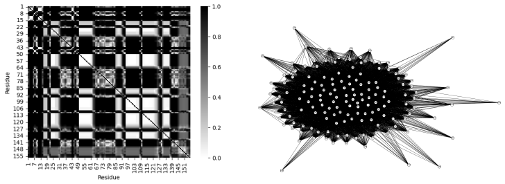
The central object is the Random Geometric Graph variable $G_{V,m}(\tau,\Sigma)$ defined on $p=156$ nodes, with the categorical state variable $X_k$ of residue $k$ attached to node $k$ and edge variables $G_{ij}$ inferred from the inter-residue absolute correlation matrix $\Sigma$ computed via Cramér's V. The edge posterior $m(G_{ij}=1|\rho_{ij})$ is derived from a $N(\rho_{ij},\nu)$ likelihood with a Bernoulli(0.5) prior on the edge and a uniform prior on $\nu$, marginalised over $\nu$. The graph is realised by setting $G_{ij}=1$ when this posterior exceeds the cut-off probability $\tau$, and the paper's 'meaningful threshold' $\tau_{\min}$ is the point where the slope of the log posterior with respect to $\tau$ is minimal, producing the 'most robust' graph. This threshold carries the $\beta$ and $\eta$ scores, while $\delta$ is computed by comparing the posterior of the full graph with the graph learned after removing one residue.
What would settle it
Compute the log posterior $\log \pi$ from Definition 2.3 at many values of $\tau$ with high precision; if the differenced slope is zero up to floating-point error, then the identified $\tau_{\min}$ and $\tau_{\max}$ are artifacts, and the $\beta$ and $\eta$ criticality rankings should be re-examined at other thresholds.
Extended reading notes
Core claim
The central claim is that critical residues of Skp1 can be identified from MD simulation data by three RGG-based scores, and that the $\delta$ parameter compares most favourably with experimental results. The graph is a random geometric graph in a probabilistic metric space: the distance between residues $i$ and $j$ is a cumulative distribution function of the disparity between the edge variable and the absolute correlation, and the edge posterior $m(G_{ij}=1|\rho_{ij})$ follows from a normal likelihood with uniform variance prior. The paper reports that the 20 residues with highest $\delta$ (largest posterior drop when removed) coincide well with experimentally tracked high-frequency state-change residues, that $\eta$ (temporal degree variability) captures several but misses residues 147--151, and that $\beta$ (full-graph degree) assigns low degree to critical residues. The threshold $\tau_{\min}$ found from minima of the slope of the log posterior is claimed to yield the most robust RGG and to be a meaningful alternative to COGENT thresholding.
Load-bearing premise
The threshold-selection procedure assumes that the log posterior of the graph varies with $\tau$ in a way that has identifiable minima and maxima, even though the paper's definition of that posterior is independent of $\tau$; if the observed slope is numerical noise, then $\tau_{\min}$ and the $\beta$ and $\eta$ scores computed at it are not well defined.
Editorial extensions
If this is right
- If the $\delta$ score is reliable, critical residues can be flagged from a single MD trajectory using only categorical state correlations, with no energy model or alignments.
- The $\tau_{\min}$ threshold rule, if valid, gives a generic replacement for arbitrary correlation cut-offs in network-based residue analysis.
- Because $\eta$ depends on the time-block size, its use requires choosing a block length matched to the interaction timescale; the paper notes an arbitrary partition did not perform best.
- Computing $\delta$ requires learning $p+1$ graph posteriors, so the method is computationally expensive for large proteins; the paper acknowledges this limitation.
- The tendency for high-$\delta$ residues to have low $\beta$ suggests the two scores could be combined into a consensus criticality ranking.
Reading between the lines
- The leave-one-out posterior difference $\delta$ might serve as a general probe for functional importance in other proteins, and the residues predicted here but not yet tested experimentally are direct candidates for mutagenesis.
- Because Cramér's V treats all eight secondary-structure states symmetrically, the method could be applied to other categorical descriptors, such as solvent exposure classes or contact maps, to test whether criticality calls are stable under alternative state definitions.
- The $\eta$ score's sensitivity to block size suggests a data-driven block-length selection, for example from the autocorrelation of the state time series, as a future improvement that the paper does not address explicitly.
Editorial analysis
A structured set of objections, weighed in public.
Referee Report
Summary. This manuscript proposes to identify critical residues of the protein Skp1 from molecular dynamics simulations by learning a random geometric graph (RGG) over 156 residue nodes. The inter-residue association matrix Sigma is computed with Cramer's V from categorical secondary-structure states, and edge probabilities are obtained from a closed-form marginal posterior. Three scores are introduced: delta, the difference between full and leave-one-residue-out graph posteriors; eta, the temporal standard deviation of nodal degree across time blocks; and beta, the nodal degree in the full graph. The paper claims that a data-driven threshold tau_min derived from the slope of the log posterior produces the 'most robust' RGG, and that the delta score identifies critical residues most favourably against experimental results. The experimental comparison is qualitative. The manuscript contains two fundamental methodological inconsistencies: the graph posterior is defined to be independent of tau while tau_min and tau_max are estimated from its derivative; and the Cramer's V computation on an N_l x 2 table measures marginal homogeneity, not pairwise temporal association. Both issues affect the validity of all three criticality scores, so the central claims in Section 3.4 are unsupported.
Significance. If the proposed method were valid, it would offer a training-free, MD-based approach to critical-residue identification, which is of practical interest for mutagenesis targeting and protein engineering. The paper does provide a self-contained derivation of the edge marginal posterior in Definition 2.2 and uses a probabilistic-metric-space formalism that is more sophisticated than simple correlation thresholding. However, the two errors identified above are not cosmetic: they invalidate the graph input and the thresholding procedure on which the method rests. The claim that delta performs best is supported only by qualitative and visual comparison, without any statistical test. Until the correlation measure and the threshold criterion are corrected and the comparison quantified, the significance of the contribution cannot be assessed.
major comments (4)
- [Definition 2.3 and Section 2.5] Definition 2.3 defines the posterior pi(G_{V,m}(tau,Sigma)|{rho_ij}) as the product over edges of m(G_ij|rho_ij), and the text explicitly states that this posterior is independent of the cut-off tau. Section 2.5 nevertheless defines tau_min and tau_max as the locations where the slope gamma(tau) = d log pi / d tau is minimal and maximal, and Section 3 reports numerical values tau_min approx 0.854 and tau_max approx 0.601. Since pi does not depend on tau, gamma(tau) is identically zero; the reported extrema are numerical artifacts of differencing noise. Because beta and eta are computed at tau_min (Sections 2.6, 2.7 and 3.2-3.3), the criticality rankings for two of the three scores are not well defined.
- [Definition 2.8 and Eq. (2.2)] The matrix Sigma is not a residue-residue correlation matrix. For a pair (X_i, X_j), Definition 2.8 forms an N_l x 2 contingency table whose two columns are the marginal state counts of X_i and X_j, and then computes Cramer's V for that table. This statistic tests whether the two marginal distributions are identical; it does not measure whether the two residues' states co-vary over time. If two residues have identical marginal distributions and perfectly synchronized states, the two columns are identical, chi^2 = 0, and rho_ij = 0, whereas the true pairwise association is maximal. Consequently, every downstream object - the edge posterior m(G_ij|rho_ij), the realised RGG, and the scores delta, eta, beta - is built from a matrix that does not represent residue-residue association. This invalidates the central claims in Section 3.4.
- [Section 3.4] The comparison with experimental critical residues is qualitative. The text states that eta 'tally moderately well' with experiments and that delta 'compares most favourably', but no overlap counts, precision/recall values, enrichment p-values, or null-model baselines are reported. There is no statistical support for the claim that delta outperforms eta or beta. A quantitative evaluation (e.g., hypergeometric enrichment of the top-n lists, or rank-based concordance) is needed before any conclusion about relative performance can be drawn.
- [Section 2.3] The graph-learning step is internally inconsistent. The algorithm samples edge variables from the closed-form posterior and then thresholds the Monte Carlo relative frequency f_ij against tau. But the posterior m(G_ij|rho_ij) is available in closed form, so the threshold should be applied directly to m(G_ij=1|rho_ij); thresholding a finite-sample frequency introduces an extra stochastic layer that is not part of the model described in Definitions 2.2-2.3. The number of samples N is not specified, so the reported graphs cannot be reproduced.
minor comments (7)
- [Throughout] The manuscript contains numerous typographical errors, including 'constrcuting' (Section 2.5), 'tecchnique' (Section 2.5), 'coloumn' (Section 3.3), 'depicetd' (Figure 7 caption), 'respcetive' (Section 2.5), 'infedilty' (Section 3.2), 'exccept' (Section 2.4), 'betweeb' (Section 2.2), and 'ecach' (Section 3.2). The manuscript would benefit from careful proofreading.
- [Definition 2.6] The sum for eta_c uses the index i with the condition i != c, but the summation runs over blocks b = 1, ..., N_b, not over residues. This notational slip should be corrected.
- [Figure 6] The table caption says that 'shaded residues indicated themselves to be identified by all measures,' but no shading legend is provided; please add a legend explaining what the shading means.
- [Definition 2.2] The Normal model for |R_ij| places positive density outside the interval [0,1], since |R_ij| is a correlation coefficient or Cramer's V value on [0,1]. The support issue should be addressed or the model replaced by a truncated distribution.
- [Section 2.6 and Figure 5] The manuscript states N_b = 21 blocks, but N_T = 10006 is not divisible by 21, so the block size N_eta would not be an integer. Please specify how the remaining rows are handled.
- [Algorithm 1 and Section 2.3] Algorithm 1 loops r from 1 to N but N is never defined. Please state the number of rejection-sampling iterations and the acceptance rate.
- [Section 2.1] The first and last residues were dropped because they 'did not undergo any change' during the simulation; the rationale for excluding non-varying residues should be stated, since a non-varying residue may itself be functionally critical and its exclusion could bias the analysis.
Circularity Check
No significant circularity: the criticality scores are computed from MD-derived correlations and compared with independent experimental data; identified flaws are correctness issues, not input-to-prediction reductions.
full rationale
The criticality pipeline is self-contained: correlations are estimated from MD state trajectories (Section 2.8), the edge posterior is computed in closed form from an explicit Normal observation model (Definition 2.2), and the three scores δ, η, β are direct functionals of the resulting graph (Definitions 2.4, 2.6, 2.7). The threshold τ_min is selected from the data via the slope of the log posterior (Section 2.5), rather than from the experimental critical-residue labels; the block size in Section 2.6 is chosen before any experimental comparison; and the experimental critical residues are external laboratory results (Reddy et al. 2018). No parameter is fitted to the experimental outcome and then reported as a prediction. The self-citations to Chakrabarty et al. (2023) and Zhang et al. (2024) are not load-bearing, because the definitions and formulas needed for the RGG construction are reproduced in this manuscript. There are genuine mathematical concerns: the contingency table in Definition 2.8 is Nℓ×2 and Eq. (2.2) measures marginal homogeneity rather than pairwise association, and the claim that the Definition 2.3 posterior is τ-independent sits awkwardly with the slope computation in Section 2.5. However, these are correctness or internal-consistency problems, not circular reductions in which a predicted quantity is equivalent to its input by construction.
Assumptions & free parameters
free parameters (4)
- Threshold probability tau_min =
0.854
- Threshold probability tau_max =
0.601
- Block size for temporal degree =
21 blocks (N_eta unspecified)
- Number of top critical residues n =
20
assumptions (5)
- ad hoc to paper Edges of the RGG are included independently of one another (Definition 2.3).
- ad hoc to paper The absolute Cramer's V correlation |R_ij| follows a Normal density with mean g_ij (0 or 1) and unknown variance.
- ad hoc to paper The slope of the log posterior with respect to tau has meaningful minima and maxima that locate robust and sensitive graphs.
- domain assumption A residue's criticality is monotonically related to temporal instability or low degree in the RGG.
- domain assumption The MD simulation states and the experimental critical residue set are reliable ground truth.
Cite this review
Pith. "Pith review of Identifying critical residues of a protein using meaningfully-thresholded Random Geometric Graphs." pith.science (2026). https://pith.science/paper/ZIN2R4J6
@misc{pith2026250610015,
  author       = {Pith},
  title        = {Pith review of: Identifying critical residues of a protein using meaningfully-thresholded Random Geometric Graphs},
  year         = {2026},
  howpublished = {\url{https://pith.science/paper/ZIN2R4J6}},
  note         = {Machine review of arXiv:2506.10015}
}
read the original abstract
Identification of critical residues of a protein is actively pursued, since such residues are essential for protein function. We present three ways of recognising critical residues of an example protein, the evolution of which is tracked via molecular dynamical simulations. Our methods are based on learning a Random Geometric Graph (RGG) variable, where the state variable of each of 156 residues, is attached to a node of this graph, with the RGG learnt using the matrix of correlations between state variables of each residue-pair. Given the categorical nature of the state variable, correlation between a residue pair is computed using Cramer's V. We advance an organic thresholding to learn an RGG, and compare results against extant thresholding techniques, when parametrising criticality as the nodal degree in the learnt RGG. Secondly, we develop a criticality measure by ranking the computed differences between the posterior probability of the full graph variable defined on all 156 residues, and that of the graph with all but one residue omitted. A third parametrisation of criticality informs on the dynamical variation of nodal degrees as the protein evolves during the simulation. Finally, we compare results obtained with the three distinct criticality parameters, against experimentally-ascertained critical residues.
Figures


Figures from the paper (4 more)


Reference graph
Works this paper leans on
-
[1]
M., Grassi, E., Damasco, C., Silengo, L., Oti, M., Provero, P., and Cunto, F
Ala, U., Piro, R. M., Grassi, E., Damasco, C., Silengo, L., Oti, M., Provero, P., and Cunto, F. D. (2008). Prediction of human disease genes by human-mouse conserved coexpression analysis. PLoS Computational Biology , 4(3):e1000043
work page 2008
-
[2]
Antonio del Sol, Florencio Pazos, A. V. (2003). Automatic methods for predicting functionally important residues. Journal of Molecular Biology , 326(4):1289–1302
work page 2003
-
[3]
Antonio del Sol, P. O. (2005). Small-world network approach to identify key residues in protein-protein interaction. Proteins , 58(3):672–682
work page 2005
-
[4]
S., Bullmore, E., Verchinski, B
Bassett, D. S., Bullmore, E., Verchinski, B. A., Mattay, V. S., Weinberger, D. R., and Meyer-Lindenberg, A. (2008). Hierarchical organization of human cortical networks in health and schizophrenia. Journal of Neuroscience , 28(37):9239--9248
work page 2008
-
[5]
Boris Thibert, Dale E Bredesen, G. d. R. (2005). Improved prediction of critical residues for protein function based on network and phylogenetic analyses. BMC Bioinformatics , 6(213)
work page 2005
-
[6]
V., Pardo-Diaz, J., Reinert, G., and Deane, C
Bozhilova, L. V., Pardo-Diaz, J., Reinert, G., and Deane, C. M. (2020). COGENT: evaluating the consistency of gene co-expression networks . Bioinformatics , 37(13):1928--1929
work page 2020
-
[7]
Capra, J. A. and Singh, M. (2007). Predicting functionally important residues from sequence conservation. Bioinformatics , 23(15):1875--1882
work page 2007
-
[8]
Chakrabarty, D. (2024). Learning in the Absence of Training Data . Springer International Publishing
work page 2024
Show all 43 references
-
[9]
Chakrabarty, D., Wang, K., Roy, G.and Bhojgaria, A., Zhang, C., Pavlu, J., and Chakrabartty, J. (2023). Constructing training set using distance between learnt graphical models of time series data on patient physiology, to predict disease scores. PloS one , 18(10):e0292404
2023
-
[10]
Cram \'e r, H. (1946). Mathematical Methods of Statistics . Chpater 21. Princeton University Press
1946
-
[11]
Crean, P
Dariia Yehorova, Rory M. Crean, P. M. K. S. C. L. K. (2024). Key interaction networks: Identifying evolutionarily conserved non-covalent interaction networks across protein families. Protein Science , 33(3):e4911
2024
-
[12]
S., and Jones, D
Drakesmith, M., Caeyenberghs, K., Dutt, A., Lewis, G., David, A. S., and Jones, D. K. (2015). Overcoming the effects of false positives and threshold bias in graph theoretical analyses of neuroimaging data. NeuroImage , 118:313--333
2015
-
[13]
Elcock, A. H. (2001). Prediction of functionally important residues based solely on the computed energetics of protein structure. Journal of Molecular Biology , 312(4):885--896
2001
-
[14]
C., Goldovsky, L., Brosch, M., van Dongen, S., Mazi \`e re, P., Grocock, R
Freeman, T. C., Goldovsky, L., Brosch, M., van Dongen, S., Mazi \`e re, P., Grocock, R. J., Freilich, S., Thornton, J., and Enright, A. J. (2007). Construction, visualisation, and clustering of transcription networks from microarray expression data. PLoS Computational Biology ...
2007
-
[15]
Gilbert, E. N. (1961). Random plane networks. Journal of the Society for Industrial and Applied Mathematics , 9(4):533--543
1961
-
[16]
P., Dettmann, C
Giles, A. P., Dettmann, C. P., and Georgiou, O. (2016). Connectivity of soft random geometric graphs over annuli. J Stat Phys , 162:1068--1083
2016
-
[17]
A., Ingraham, J
Hopf, T. A., Ingraham, J. B., Poelwijk, F. J., Schärfe, C. P. I., Springer, M., Sander, C., and Marks, D. S. (2017). Mutation effects predicted from sequence co-variation. Nature Biotechnology , 35(2):128–135
2017
-
[18]
F., Asteriou, V., Papadimitriou-Tsantarliotou, A., Petrou, A., Angelis, L., Nicopolitidis, P., Papadimitriou, G., and Vizirianakis, I
Kantelis, K. F., Asteriou, V., Papadimitriou-Tsantarliotou, A., Petrou, A., Angelis, L., Nicopolitidis, P., Papadimitriou, G., and Vizirianakis, I. S. (2022). Graph theory-based simulation tools for protein structure networks. Simulation Modelling Practice and Theory , 121:102640
2022
-
[19]
Lockless, S. W. and Ranganathan, R. (1999). Evolutionarily conserved pathways of energetic connectivity in protein families. Science , 286(5438):295--299
1999
-
[20]
Manming Xu, Sarath Chandra Dantu, J. A. G. R. A. B. A. P. S. H. (2025). Functionally important residues from graph analysis of coevolved dynamic couplings. eLife , 14:RP105005
2025
-
[21]
Menger, K. (1942). Statistical metrics. Proc Natl Acad Sci U S A. , 28(12):535–537
1942
-
[22]
Cusack, Boris Thibert, D
Michael P. Cusack, Boris Thibert, D. E. B. G. d. R. (2007). Efficient identification of critical residues based only on protein structure by network analysis. PLoS ONE , 2(5):e421
2007
-
[23]
Nadezhda T Doncheva, Yassen Assenov, F. S. D. M. A. (2012). Topological analysis and interactive visualization of biological networks and protein structures. Nat Protoc , 7:670–685
2012
-
[24]
Nevin Gerek, Z., Kumar, S., and Banu Ozkan, S. (2013). Structural dynamics flexibility informs function and evolution at a proteome scale. Evolutionary Applications , 6(3):423--433
2013
-
[25]
Nurit Haspel, F. J. (2017). Methods for detecting critical residues in proteins. In Vitro Mutagenesis , 1498:227–242
2017
-
[26]
Osuna, S. (2020). The challenge of predicting distal active site mutations in computational enzyme design. WIREs Computational Molecular Science , 11(3):e1502
2020
-
[27]
S., Beguerisse-Díaz, M., Deane, C
Pardo-Diaz, J., Poole, P. S., Beguerisse-Díaz, M., Deane, C. M., and Reinert, G. (2022). Generating weighted and thresholded gene coexpression networks using signed distance correlation . Network science (Cambridge University Press) , 10(2):131--145
2022
-
[28]
Penrose, M. D. (2016). Connectivity of soft random geometric graphs. The Annals of Applied Probability , 26(2):986--1028
2016
-
[29]
Perkins, A. D. and Langston, M. A. (2009). Threshold selection in gene co-expression networks using spectral graph theory techniques. BMC Bioinformatics , 10(Suppl 11):S4
2009
-
[30]
Rebecca Hamer, Qiang Luo, J. P. A. G. R. C. M. D. (2010). i-patch: interprotein contact prediction using local network information. Proteins , 78(13):2781–2797
2010
-
[31]
G., Pratihar, S., Ban, D., Frischkorn, S., Becker, S., Griesinger, C., and Lee, D
Reddy, J. G., Pratihar, S., Ban, D., Frischkorn, S., Becker, S., Griesinger, C., and Lee, D. (2018). Simultaneous determination of fast and slow dynamics in molecules using extreme cpmg relaxation dispersion experiments. Journal of Biomolecular NMR , 70:1--9
2018
-
[32]
and Schneider, R
Sander, C. and Schneider, R. (1991). Database of homology-derived protein structures and the structural meaning of sequence alignment. Proteins: Structure, Function, and Bioinformatics , 9(1):56--68
1991
-
[33]
Schulman, B.A.and Carrano, A. J. P. B. Z. K. E. F. M. E. S. H. J. P. M. P. N. (2000). Insights into scf ubiquitin ligases from the structure of the skp1-skp2 complex. Nature , 408:381--386
2000
-
[34]
and Sklar, A
Schweizer, B. and Sklar, A. (2011). Probabilistic Metric Spaces . Dover Publications
2011
-
[35]
S., Erman, B., and Mastrandrea, L
Shenkin, P. S., Erman, B., and Mastrandrea, L. D. (1991). Information-theoretical entropy as a measure of sequence variability. Proteins , 11(4):297--313
1991
-
[36]
G., Xu, X
Su, J. G., Xu, X. J., Li, C. H., Chen, W. Z., and Wang, C. X. (2011). Identification of key residues for protein conformational transition using elastic network model. The Journal of Chemical Physics , 135(17):174101
2011
-
[37]
J., and Leibler, S
Teşileanu, T., Colwell, L. J., and Leibler, S. (2015). Protein sectors: Statistical coupling analysis versus conservation. PLoS Comput Biol. , 11(2)
2015
-
[38]
Theis, N., Rubin, J., Cape, J., Iyengar, S., and Prasad, K. M. (2023). Threshold selection for brain connectomes. Brain Connectivity , 13(7):441--455
2023
-
[39]
Cover, J
Thomas M. Cover, J. A. T. (1991). Elements of Information Theory , pages 510--525. John Wiley & Sons, Ltd
1991
-
[40]
Watts, D. J. and Strogatz, S. H. (1998). Collective dynamics of 'small-world' networks. Nature , 393(6684):440--442
1998
-
[41]
A., Szurmant, H., Hoch, J
Weigt, M., White, R. A., Szurmant, H., Hoch, J. A., and Hwa, T. (2009). Identification of direct residue contacts in protein–protein interaction by message passing. Proceedings of the National Academy of Sciences , 106(1):67--72
2009
-
[42]
N., and Barahona, M
Wu, N., Yaliraki, S. N., and Barahona, M. (2022). Prediction of protein allosteric signalling pathways and functional residues through paths of optimised propensity
2022
-
[43]
Zhang, C., Grosan, C., and Chakrabarty, D. (2024). Individualised recovery trajectories of patients with impeded mobility, using distance between probability distributions of learnt graphs. Artificial Intelligence in Medicine , 157:103005
2024
Reviewed August 7, 2026 · model on record in the stance chip above.
Discussion (0). Sign in to comment.