REVIEW 3 major objections 5 minor 38 references
Statistical mechanics of fluids with hidden degrees of freedom
T0 review · 3 major / 5 minor · reviewed 2026-08-07 · deepseek-v4-flash
Pith's one-line read The paper claims that fluids whose molecules carry hidden degrees of freedom can form droplet-like density patterns of finite length scale in thermal equilibrium, with no continuous energy input.
desk verdict A genuinely new equilibrium mechanism for finite-length-scale patterns, but the numerical evidence samples the wrong ensemble, the sign of the free-energy correction looks inconsistent, and the convexity proof has a gap. read the letter →
The pith
A machine-rendered reading of the paper's core claim, the machinery that carries it, and where it could break.
The reading
What carries the argument
The central object is the separation of molecular degrees of freedom into external $\sigma$ (which interact through pair potentials), internal $\tau$ (which enter only through the single-particle potential), and an underlying field $\lambda$ that mediates the single-particle potential, together with the 2+2-state model, a minimal model with one binary external state and one binary internal state per particle. The working identity is the saddle-point structure of the grand potential: minimizing over $\lambda$ gives the effective free-energy contribution $F'_\beta[\rho] = -\int dr\,d\sigma\,\rho_{\mathrm{ex}}(r,\sigma)\,\nu^\dagger[\rho]$, which converts the equilibrium condition into a modified stationarity equation. In the 2+2-state model the specific coupling $\varepsilon = (u_\sigma + u_\tau \hat{T})\lambda$ with a self-adjoint operator $\hat{T}$ yields the explicit relation $\beta\lambda = \hat{T}^{-1}\operatorname{arctanh}(\rho_{\mathrm{tot}}^{-1}\hat{T}^{-1}\Delta\rho)$, and substituting this relation produces the stationary Allen-Cahn and Cahn-Hilliard equations with linear reaction terms that carry the paper's main results.
What would settle it
A concrete test: in a sealed, thermally equilibrated binary fluid whose molecules have two internal conformational states, measure the density correlation length as a function of system size at decreasing temperature; if the correlation length diverges with system size instead of saturating at a finite value, the predicted absence of a true phase transition and the equilibrium finite-length patterns are contradicted.
Extended reading notes
Core claim
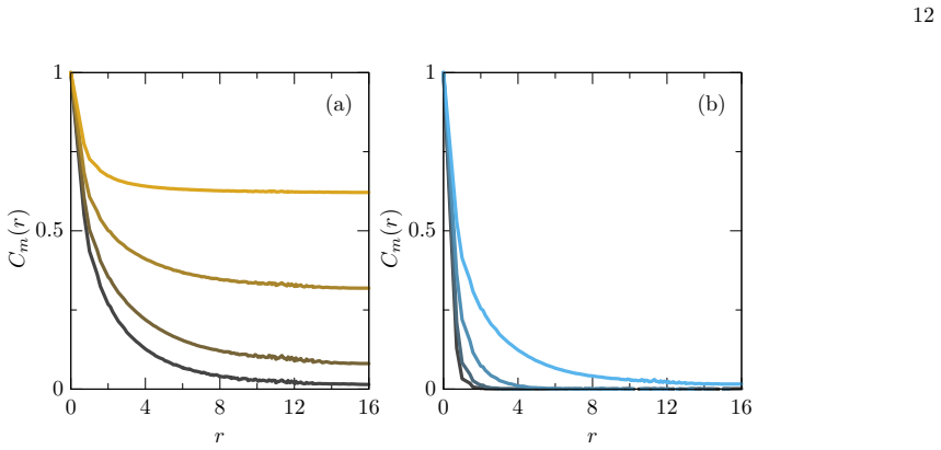
The paper derives an equilibrium statistical mechanics for fluids with hidden degrees of freedom. The grand potential is minimized jointly over the density profile and the underlying field $\lambda$, and eliminating $\lambda$ produces a total free energy $F_\beta[\rho] + F'_\beta[\rho]$ in which the hidden degrees of freedom generate a "pseudo-driving force" that deforms the equilibrium of the visible system. In the 2+2-state model, where each particle has one external and one internal two-state variable coupled by $\varepsilon = (u_\sigma + u_\tau \hat{T})\lambda$, the minimization reduces exactly to the stationary Allen-Cahn equation with a linear reaction term when $\hat{T}$ is constant, and to the stationary Cahn-Hilliard equation with a linear reaction term when $\hat{T}^2 = -(\rho_{\mathrm{tot}}/\alpha')\nabla^2$. Because these equations are obtained from a minimum principle rather than from a prescribed time evolution, their patterned solutions describe equilibrium states, not steady states of an active system. Monte Carlo simulations of the lattice version confirm the absence of a continuous phase transition and show heterogeneous density profiles whose correlation length stays finite while growing as the reaction probability decreases.
Load-bearing premise
The load-bearing premise is that the underlying degree of freedom $\lambda$ sits in thermal equilibrium with the fluid, so the free energy is minimized with respect to $\lambda$; the coupling form $\varepsilon = (u_\sigma + u_\tau \hat{T})\lambda$ is chosen by hand rather than derived from molecular structure, and if $\lambda$ is actually held out of equilibrium by chemical energy, the equilibrium free-energy argument does not apply.
Editorial extensions
If this is right
- The stationary Allen-Cahn and Cahn-Hilliard equations with linear reaction terms, long used as non-equilibrium models, also characterize equilibrium states of a class of microscopic Hamiltonians, so patterned solutions of those equations are not by themselves evidence of energy input.
- Equilibrium microphase separation with a finite correlation length is possible without any chemical reaction or external drive, because hidden internal states supply the effective coupling that stabilizes the pattern.
- Observed droplet patterns in cells cannot be taken as proof of non-equilibrium steady states; the same appearance can arise from equilibrium hidden degrees of freedom.
- The hidden-DOF free energy term makes the total free energy strongly convex, so the finite-length-scale structures appear without the fine-tuning of temperature that a critical point would require.
Reading between the lines
- A testable extension the paper leaves implicit: if the hidden field $\lambda$ relaxes slowly compared with experimental timescales, systems could look active simply because they have not yet reached the assumed equilibrium state; measuring $\lambda$ directly would distinguish this from genuine non-equilibrium driving.
- The same variational machinery suggests that other linear-reaction pattern-forming equations, including those with fractional Laplacian couplings, could describe equilibrium states of fluids with fractal or porous internal structure; this is a natural next case to check.
- In chemically active droplet experiments, ATP consumption might serve to keep the underlying field $\lambda$ out of equilibrium rather than to drive phase separation directly, which would change how such experiments are interpreted and designed.
- Pinning or externally forcing $\lambda$ in the 2+2-state model would break the equilibrium assumption and should restore the standard phase transition, giving a concrete experimental dial for testing the mechanism.
Editorial analysis
A structured set of objections, weighed in public.
Referee Report
Summary. The paper introduces a general statistical-mechanical framework for fluids with 'hidden' degrees of freedom: each particle has an external DOF σ, an internal DOF τ, and the single-particle energy depends on an underlying fluctuating field λ. After tracing out τ and minimizing over λ, the authors derive an effective free energy for the original system. They then analyze a minimal '2+2' model and claim that the equilibrium free energy acquires a positive convex contribution from the hidden DOF, which suppresses phase transitions and produces heterogeneous density profiles with a finite length scale. The stationary equations are identified with the Allen-Cahn and Cahn-Hilliard equations with linear reaction terms, and Monte Carlo simulations of a 'reactive model' are presented as numerical evidence.
Significance. If correct, the central claim would be significant: it would provide a microscopic equilibrium mechanism for finite-length-scale heterogeneity, challenging the common interpretation of such patterns as requiring non-equilibrium driving. The paper is self-contained, derives results from a Hamiltonian without fitted experimental parameters, and connects to a substantial literature on active droplets and microphase separation. These strengths are real. However, the central conclusion depends on the sign of a Legendre transform and on a Monte Carlo algorithm that does not sample the claimed equilibrium ensemble. Both are load-bearing problems, and the strong-convexity proof additionally assumes convexity of the very free energy that the paper wants to apply it to. The significance of the paper therefore cannot be established in its current form.
major comments (3)
- [Sec. II.B, Eqs. (2.14)-(2.17), (2.21); Sec. III.A.1, Eq. (3.15)] The sign of the Legendre transform is wrong and propagates into the model. From Eqs. (2.12)-(2.14), integrating out τ and performing the saddle point in λ gives βΦ = min_{ρ,λ} (βFβ + ∫ρβν), so the minus sign in Eq. (2.16) is an error; the correct Euler equation is δβFβ/δρ + βν = 0, not Eq. (2.17). For the 2+2 model, βν_A - βν_B = 2βλ and the thermodynamic identity gives ∫ρβν = -βF^free at the optimum, so the physical total free energy is βFβ - βF^free, not βFβ + βF^free as used in Eq. (3.15). Consequently Eq. (3.20) should read δβFβ/δΔρ - α²Δρ = 0, the equivalence to the Allen-Cahn equation with a linear reaction term in Eq. (3.21) is lost, and the strong-convexity argument in Eqs. (3.25)-(3.26) does not apply. Since the paper's central claim of suppressed phase separation depends on this sign, the error is load-bearing.
- [Sec. III.A.2, Eqs. (3.27)-(3.31), Figs. 1-4] The Monte Carlo algorithm does not sample the equilibrium of the effective free energy F_tot. The reaction step flips a spin with probability p without Metropolis acceptance; composing this symmetric flip generator with Metropolis updates for H_Ising violates detailed balance with respect to any local Hamiltonian. For a spin flip with Ising energy change ΔE, detailed balance would require an effective energy change f(ΔE) satisfying f(ΔE) = -f(-ΔE), but the algorithm's transition rates give f(ΔE) = -(1/β)log[(e^{-βΔE}+p/N)/(1+p/N)] for energy-raising flips and f(-ΔE) = (1/β)log[(e^{βΔE}+p/N)/(1+p/N)] for energy-lowering flips, which are not negatives for p>0. The chain is therefore a non-equilibrium steady state. The fact that the deterministic stationary equation (3.20) coincides with the stationary limit of Eq. (3.21) does not justify interpreting the fluctuations, correlation functions, and susceptibilities in Figs. 1-4 as equilibrium averages over F_tot. Thus the numerical demonstration of the central claim is invalid.
- [Sec. III.A.1, Eqs. (3.25)-(3.26)] The proof that F_tot is strongly convex assumes that the second variation of βFβ is nonnegative. This is not true for a phase-separating original system, which is precisely the case of interest and the case simulated (the Ising model below T_c). Without convexity of Fβ, the first term in Eq. (3.26) can be negative and can dominate the positive α² term, so the inequality fails and the claim that the system has no continuous phase transition for any α≠0 is not established. This is a load-bearing gap because the paper's qualitative conclusions are drawn for systems whose original free energy is non-convex.
minor comments (5)
- [Throughout] The symbol T is used both for the temperature and for the operator T̂ in the 2+2 model; please use distinct notation to avoid confusion.
- [Sec. III.A, Eq. (3.31)] The susceptibility is defined with ⟨|m|⟩ rather than ⟨m⟩; this is unconventional and should be justified, especially because in a non-equilibrium steady state the fluctuation-response relation implicit in this definition may not hold.
- [Sec. III.A.1, after Eq. (3.21)] The statement that Eq. (3.21) 'can be interpreted as an algorithm to sample equilibrium states' is misleading; a valid equilibrium sampling algorithm would need to implement detailed balance for F_tot, which the reactive model does not do.
- [Sec. III, Eq. (3.5)] The specific coupling ε[r,σ,τ|λ] = (u_σ + u_τ T̂)λ and the choice T̂² = -(ρ_tot/α')∇² for microphase separation are introduced by hand; a discussion of how such couplings might arise from molecular structure would improve the physical motivation.
- [Sec. II.A, Assumption 2'] Assumption 2' states that λ is in thermal equilibrium with the fluid and is minimized or integrated out; this is a strong assumption for biological contexts where the underlying DOF may be driven by chemical energy, and the paper would benefit from a more explicit statement of the validity regime.
Circularity Check
No significant circularity; the core derivation is self-contained, with only a minor non-load-bearing self-citation and a simulation-validation concern that is not a circularity.
full rationale
The central derivation is self-contained: starting from the Hamiltonian (2.8) under Assumptions 1 and 2', the paper computes the grand potential (2.12), performs the Legendre transform (2.13), and evaluates the saddle point over the underlying field λ (2.14), giving the effective free energy F_tot = F_β + F'_β in Eq. (2.19). The specific forms in Sec. III, Eqs. (3.14)-(3.17) and Eq. (3.33), follow algebraically from the chosen coupling ε = (u_σ + u_τ T̂)λ. The choices T̂ = const. and T̂² = -(ρ_tot/α')∇² are explicit modeling assumptions, not quantities fitted to the target Allen-Cahn or Cahn-Hilliard behavior, and the paper does not claim to derive them from molecular structure. The stated equivalence between Eq. (3.20) and the stationary Allen-Cahn equation (3.21), and between Eq. (3.33) and the stationary Cahn-Hilliard equation (3.34), is an identity of stationarity conditions; this is a constructive existence result rather than a circular reduction, because the target equation is not used as an input to derive itself. The only self-citation, Ref. [29], is an illustrative example motivating Assumption 2 and is not load-bearing. A separate correctness concern is that the Monte Carlo 'reaction step' in Sec. III A 2 flips spins without a Metropolis acceptance test, so the simulated reactive model may not sample the Boltzmann weight of F_tot; this undermines the numerical demonstration but is not an instance of circular reasoning.
Assumptions & free parameters
free parameters (4)
- α (Allen-Cahn case) =
not fitted
- α' (Cahn-Hilliard case) =
not fitted
- Operator T̂ =
constant or -(ρ_tot/α')∇²
- p (reaction probability) =
0.1, 0.2, 0.5
assumptions (5)
- domain assumption Assumption 1 (Separability of DOF): each particle has external DOF σ interacting via pair potential and internal DOF τ appearing only in the single-particle potential.
- domain assumption Assumption 2' (Mean-field equilibrium of λ): the single-particle potential ε depends on a time-independent underlying DOF λ, and the system is in equilibrium including λ, so the free energy is minimized with respect to λ.
- standard math Saddle-point (Laplace) approximation for the λ integral in Eq (2.12).
- domain assumption Incompressibility condition ρ_A + ρ_B = constant.
- ad hoc to paper Convexity of the original free energy Fβ.
invented entities (1)
-
Underlying DOF field λ(r,σ,τ)
Cite this review
Pith. "Pith review of Statistical mechanics of fluids with hidden degrees of freedom." pith.science (2026). https://pith.science/paper/NBQ3UDCJ
@misc{pith2026250610253,
  author       = {Pith},
  title        = {Pith review of: Statistical mechanics of fluids with hidden degrees of freedom},
  year         = {2026},
  howpublished = {\url{https://pith.science/paper/NBQ3UDCJ}},
  note         = {Machine review of arXiv:2506.10253}
}
read the original abstract
Although coarse-grained models have been widely used to explain exotic phenomena in complex fluids, such as droplet formation in living cells, these conventional approaches often fail to capture the intricate microscopic degrees of freedom that such fluids inherently possess. In this study, we propose a model that incorporates distinct microscopic degrees of freedom and their interactions, without directly relying on conventional coarse-grained descriptions. By introducing two key assumptions, we show that the system can exhibit equilibrium states characterized by heterogeneous density profiles with finite length scales, resembling those typically associated with non-equilibrium phenomena. These findings highlight the importance of distinguishing between equilibrium states and non-equilibrium steady states in highly complex systems.
Figures


Figures from the paper (1 more)
Reference graph
Works this paper leans on
-
[1]
Theory Assume that ˆT is a constant. We have from Eq. (3.17) and (3.18) βΦβ[εστ [r|λ]] = min ∆ρex(r),∆ρaux(r)√ ρtot∆ρaux(r)=α∆ρex(r) βFβ[∆ρex(r)] + βF free β [∆ρaux(r)] , (3.19) 0 = δβFβ[∆ρex(r)] δ∆ρex(r) + α2∆ρex(r), (3.20) where α := p 1/ρtot ˆT −1. The expression in Eq. (3.20) is equivalent to the stationary limit of the Allen-Cahn equation with a line...
-
[2]
Simulation We performed Monte Carlo simulations of this version of the 2+2–state model, which will be called the “reactive model” only in this subsection for convenience. To this end, we utilized the expression in Eq. (3.20) and replaced the original free energy Fβ by that of the binary lattice-gas model, or equivalently, the ferromagnetic Ising model F I...
-
[3]
When ˆT 2 = −(ρtot/α′)∇2, we have from Eq
Theory In this subsection, we consider a slightly different version of the 2+2–state model to relate our theory to previous studies on models that exhibit microphase separation. When ˆT 2 = −(ρtot/α′)∇2, we have from Eq. (3.18) 0 = ∇2 δβFβ[∆ρex(r)] δ∆ρex(r) − α′∆ρex(r), (3.33) which is equivalent to the stationary limit of the Cahn-Hillard equation with a...
-
[4]
(3.34) [20–27] and a comparison of our results with those gives some insights into our model
Comparison with previous studies There are many theoretical and numerical studies on Eq. (3.34) [20–27] and a comparison of our results with those gives some insights into our model. Before explaining the complications that arise when physically interpreting Eq. (3.34), we summarize some of its mathematical aspects regarding the stationary states, which w...
-
[5]
R. G. Larson, The structure and rheology of complex fluids , Topics in Chemical Engineering (Oxford University Press, New York, NY, 1998). 16
work page 1998
-
[6]
J. Hansen and I. McDonald, Theory of Simple Liquids , 4th ed. (Elsevier Science, 2013)
work page 2013
-
[7]
R. P. Sear and J. A. Cuesta, Phys. Rev. Lett. 91, 245701 (2003), arXiv:cond-mat/0307326 [cond-mat.soft]
work page Pith review arXiv 2003
-
[8]
S. F. Banani, H. O. Lee, A. A. Hyman, and M. K. Rosen, Nature Reviews Molecular Cell Biology 18, 285 (2017)
work page 2017
Show all 38 references
-
[9]
P. E. Wright and H. Dyson, Journal of Molecular Biology 293, 321 (1999)
1999
-
[10]
V. N. Uversky, J. R. Gillespie, and A. L. Fink, Proteins: Structure, Function, and Bioinformatics 41, 415 (2000)
2000
-
[11]
Dunker, J
A. Dunker, J. Lawson, C. J. Brown, R. M. Williams, P. Romero, J. S. Oh, C. J. Oldfield, A. M. Campen, C. M. Ratliff, K. W. Hipps, J. Ausio, M. S. Nissen, R. Reeves, C. Kang, C. R. Kissinger, R. W. Bailey, M. D. Griswold, W. Chiu, E. C. Garner, and Z. Obradovic, Journal of Mole...
2001
-
[12]
Tompa, Trends in Biochemical Sciences 27, 527 (2002)
P. Tompa, Trends in Biochemical Sciences 27, 527 (2002)
2002
-
[13]
Wells, H
M. Wells, H. Tidow, T. J. Rutherford, P. Markwick, M. R. Jensen, E. Mylonas, D. I. Svergun, M. Blackledge, and A. R. Fersht, Proceedings of the National Academy of Sciences 105, 5762 (2008)
2008
-
[14]
P. Li, S. Banjade, H.-C. Cheng, S. Kim, B. Chen, L. Guo, M. Llaguno, J. V. Hollingsworth, D. S. King, S. F. Banani, P. S. Russo, Q.-X. Jiang, B. T. Nixon, and M. K. Rosen, Nature 483, 336 (2012)
2012
-
[15]
V. N. Uversky, I. M. Kuznetsova, K. K. Turoverov, and B. Zaslavsky, FEBS Letters 589, 15 (2015)
2015
-
[16]
A. A. Hyman and C. P. Brangwynne, Developmental Cell 21, 14 (2011)
2011
-
[17]
A. A. Hyman, C. A. Weber, and F. J¨ ulicher, Annu Rev Cell Dev Biol 30, 39 (2014)
2014
-
[18]
C. F. Lee, C. P. Brangwynne, J. Gharakhani, A. A. Hyman, and F. J¨ ulicher, Phys. Rev. Lett. 111, 088101 (2013)
2013
-
[19]
Shelest, H
A. Shelest, H. L. Roy, D. M. Busiello, and P. D. L. Rios, arXiv:2406.19266 [physics.bio-ph]
-
[20]
Vweza, C.-G
A.-O. Vweza, C.-G. Song, and K.-T. Chong, International Journal of Molecular Sciences 22 (2021)
2021
-
[21]
Zwicker, Current Opinion in Colloid & Interface Science 61, 101606 (2022), arXiv:2202.13646 [cond-mat.soft]
D. Zwicker, Current Opinion in Colloid & Interface Science 61, 101606 (2022), arXiv:2202.13646 [cond-mat.soft]
2022 arXiv
- [22]
-
[23]
Zwicker, M
D. Zwicker, M. Decker, S. Jaensch, A. A. Hyman, and F. J¨ ulicher, Proceedings of the National Academy of Sciences 111, E2636 (2014)
2014
-
[24]
Ohta and K
T. Ohta and K. Kawasaki, Macromolecules 19, 2621 (1986)
1986
-
[25]
S. C. Glotzer, D. Stauffer, and N. Jan, Phys. Rev. Lett. 72, 4109 (1994)
1994
-
[26]
S. C. Glotzer and A. Coniglio, Phys. Rev. E 50, 4241 (1994)
1994
-
[27]
S. C. Glotzer, E. A. Di Marzio, and M. Muthukumar, Phys. Rev. Lett. 74, 2034 (1995)
1995
-
[28]
Lefever, D
R. Lefever, D. Carati, and N. Hassani, Phys. Rev. Lett. 75, 1674 (1995)
1995
-
[29]
S. C. Glotzer, D. Stauffer, and N. Jan, Phys. Rev. Lett. 75, 1675 (1995)
1995
-
[30]
Toxvaerd, Phys
S. Toxvaerd, Phys. Rev. E 53, 3710 (1996)
1996
-
[31]
Choksi, M
R. Choksi, M. A. Peletier, and J. F. Williams, SIAM Journal on Applied Mathematics 69, 1712 (2009)
2009
-
[32]
S. Laha, J. Bauermann, F. J¨ ulicher, T. C. T. Michaels, and C. A. Weber, Phys. Rev. Res.6, 043092 (2024), arXiv:2403.05228 [cond-mat.soft]
2024 arXiv
-
[33]
Kamimura, Y
A. Kamimura, Y. Sughiyama, and T. J. Kobayashi, Phys. Rev. Res. 6, 023173 (2024), arXiv:2312.14435 [cond-mat.stat- mech]
2024 arXiv
-
[34]
L. D. Landau and E. M. Lifshitz, Statistical Physics, Part 1, Course of Theoretical Physics, Vol. 5 (Butterworth-Heinemann, Oxford, 1980)
1980
-
[35]
Morita and K
T. Morita and K. Hiroike, Progress of Theoretical Physics 25, 537 (1961)
1961
-
[36]
Lischke, G
A. Lischke, G. Pang, M. Gulian, F. Song, C. Glusa, X. Zheng, Z. Mao, W. Cai, M. M. Meerschaert, M. Ainsworth, and G. E. Karniadakis, Journal of Computational Physics 404, 109009 (2020), arXiv:1801.09767 [math.NA]
2020 arXiv
-
[37]
C. A. Weber, D. Zwicker, F. J¨ ulicher, and C. F. Lee, Reports on Progress in Physics 82, 064601 (2019), arXiv:1806.09552 [cond-mat.soft]
2019 arXiv
-
[38]
H¨ anggi, P
P. H¨ anggi, P. Talkner, and M. Borkovec, Rev. Mod. Phys.62, 251 (1990)
1990
Reviewed August 7, 2026 · model on record in the stance chip above.
Discussion (0). Continue with ORCID to comment.