REVIEW 4 major objections 7 minor 74 references
A Time-Symmetric Quantum Algorithm for Direct Eigenstate Determination
T0 review · 4 major / 7 minor · reviewed 2026-08-07 · deepseek-v4-flash
Pith's one-line read Forward-backward time evolution about a preset energy is a spectral filter: it amplifies the eigenstate nearest that energy in one subspace and the farthest in the other, so any eigenstate appears without computing lower states first.
desk verdict Correct spectral-filter identity, but the 'direct' eigenstate claim is overstated: the method needs a target energy estimate and non-negligible overlap, and the numerical demos seed those inputs from known spectra. read the letter →
The pith
A machine-rendered reading of the paper's core claim, the machinery that carries it, and where it could break.
The reading
What carries the argument
The engine is the energy-shifted, time-symmetric evolution pair $U_f^{e_s}=e^{-i(H-e_s)t}$ and $U_b^{e_s}=e^{+i(H-e_s)t}$, whose sum and difference convert the Hamiltonian spectrum into a filter: $(U_f^{e_s}+U_b^{e_s})^k=[2\cos((H-e_s)t)]^k$ acts in the $\lvert 0\rangle$ ancilla subspace and $(U_f^{e_s}-U_b^{e_s})^k=[-2i\sin((H-e_s)t)]^k$ acts in the $\lvert 1\rangle$ subspace. This turns eigenvalue selection into a spectral filtering problem: after $k$ rounds the target component is amplified relative to every other component by the $k$-th power of a cosine (or sine) ratio, giving convergence exponential in $k$ and an iteration count $O(\log(1/\epsilon))$ for accuracy $\epsilon$. The non-unitary filter is realized either by expanding the Hilbert space with a control ancilla (the linear-combination-of-unitaries route, with an iteration-free variant that trades $k-1$ extra ancillas against repeated measurements) or by a quantum Monte Carlo estimator of the same cosine and sine powers, which keeps the sampling overhead polynomial rather than exponential.
What would settle it
Take a two-level system $H=\sigma_z$ with the shift exactly halfway between the levels, $e_s=0$: both eigenstates have equal factors $\cos((\pm 1)t)$, the cosine filter amplifies them identically, and the output stays the equal superposition for every $k$, so the claimed convergence to the nearest eigenstate fails whenever the nearest state is not unique. Similarly, if the initial state has zero overlap with the target, $\langle E_s|\psi_0\rangle=0$, that component remains identically zero under the filter, so overlap-blind extraction is impossible; both cases are checkable on a two-qubit device.
Extended reading notes
Core claim
The load-bearing claim is the filtering identity in Eqs. (4)--(5): writing the trial state as $\sum_i a_i \lvert E_i\rangle$, the $k$-fold application of the sum $e^{-i(H-e_s)t}+e^{+i(H-e_s)t}$ gives $\sum_i a_i [2\cos((E_i-e_s)t)]^k \lvert E_i\rangle$ in the $\lvert 0\rangle$ subspace, while the difference gives $\sum_i a_i [-2i\sin((E_i-e_s)t)]^k \lvert E_i\rangle$ in the $\lvert 1\rangle$ subspace. Provided every $(E_i-e_s)t$ lies in $[-\pi/2,\pi/2]$, the cosine factor is largest for the eigenstate nearest to $e_s$ and the sine factor is largest for the one farthest from $e_s$, so as $k$ grows those two states dominate their respective subspaces at a rate set by the ratio of the factors. The algorithm is therefore a direct eigensolver: set $e_s$ near the ground-state energy and the $\lvert 0\rangle$ subspace yields the ground state while the $\lvert 1\rangle$ subspace yields the highest excited state, giving the energy bandwidth in one run; set $e_s$ near any target eigenvalue and that eigenstate is amplified directly. Because the target is never found by first solving lower levels, the paper claims the method is free of error accumulation, and because no classical parameter optimization is involved, it cannot suffer barren plateaus.
Load-bearing premise
The scheme presupposes that the user already knows roughly where the target energy lies, so the shift $e_s$ can be set near it, and that the initial state already has a noticeable overlap with the target eigenstate; when the energy is unknown or the overlap $|a_s|^2$ is tiny, convergence slows and the Monte Carlo sampling cost, which the paper's Appendix A finds growing like $|a_s|^{-4}$, blows up.
Editorial extensions
If this is right
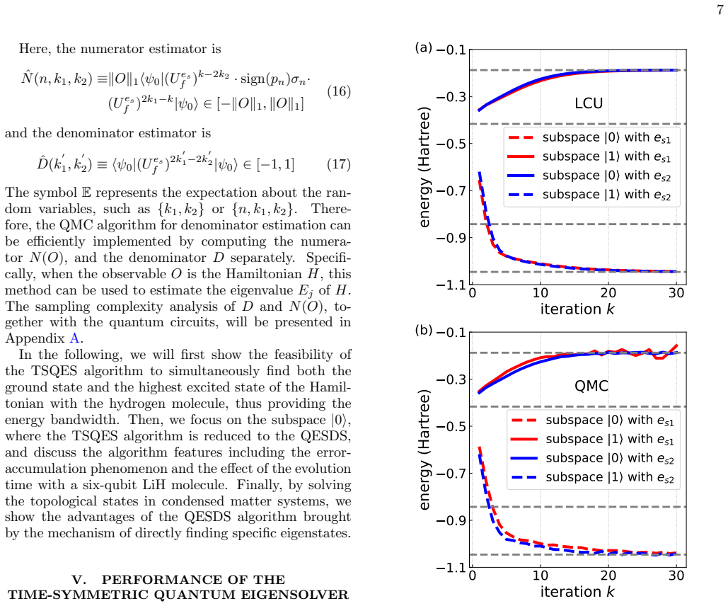
- Choosing $e_s$ near the ground-state energy yields the ground state in the $\lvert 0\rangle$ subspace and the highest excited state in the $\lvert 1\rangle$ subspace, so the energy bandwidth comes out of a single run; the hydrogen-molecule simulation reaches chemical accuracy with error $1.5\times10^{-3}$ Hartree.
- Any excited state can be targeted directly by setting $e_s$ near its energy: in the LiH study the per-level error stays flat as the level number increases, whereas the FQESS comparison shows errors growing with level number, demonstrating that the direct scheme avoids error accumulation.
- Convergence is exponential in the iteration count $k$, with $O(\log(1/\epsilon))$ iterations needed for accuracy $\epsilon$, and the absence of classical optimization removes the barren-plateau problem of variational eigensolvers.
- The quantum Monte Carlo implementation avoids the exponential post-selection decay of the LCU route, keeping sample counts polynomial with a leading dependence of order $|a_s|^{-4}$ and circuit depth low, which the authors argue suits near-term hardware.
- The solver detects topological phase transitions from gap-edge data alone: it reproduces the Kane-Mele edge states for mass $M=0$ and their disappearance for $M=0.4$, and it locates the SSH+Hubbard transition where the ground-state degeneracy changes and the energy gap closes.
Reading between the lines
- Editorial: because the convergence ratio depends on $t$ as well as on $e_s$, sweeping $e_s$ across the spectrum, one run per value, would turn the solver into a general spectral probe that maps band structure point by point, a use the paper only gestures at in its flat-band demonstrations.
- Editorial: the filter amplifies equally any two eigenstates placed symmetrically around $e_s$, so combining two or more evolution times, for example a short $t$ to separate near-degenerate pairs, is a natural extension for resolving degeneracies that a single $t$ cannot split; the paper does not test this regime.
- Editorial: the pipeline the paper itself adopts for the SSH+Hubbard case, seeding $e_s$ and the initial state from the non-interacting solution, suggests the algorithm's most realistic role is state refinement and gap detection inside a hybrid classical-quantum workflow rather than first-principles spectral discovery.
Editorial analysis
A structured set of objections, weighed in public.
Referee Report
Summary. The paper proposes TSQES, a nonvariational quantum algorithm for eigenstate determination that interferes forward and backward time evolution with an energy shift e_s. The central identity, Eq. (4), expands the k-fold filtered state in the |0> subspace as sum_i a_i [2 cos((E_i-e_s)t)]^k |E_i>, so the eigenstate closest to e_s dominates with increasing k; Eq. (5) gives the sine analogue for the eigenstate farthest from e_s. The authors present LCU and QMC implementations, an iteration-free version using additional ancillas, and numerical demonstrations for H2, LiH, the Kane-Mele model, the SSH model with Hubbard interaction, and twisted bilayer graphene. The paper claims simultaneous ground/highest-excited-state determination, direct extraction of arbitrary eigenstates without computing lower states, and avoidance of error accumulation.
Significance. If the claims were fully supported, the paper would offer a simple spectral filter that avoids the barren-plateau problem and error accumulation of variational and sequential excited-state methods. The mathematical core, Eq. (4), is a correct expansion, and the paper provides explicit circuits, a QMC sampling strategy, and several numerical studies. The main value is as a nonvariational eigenstate filter conditioned on an energy estimate and on initial-state overlap. However, the paper's stronger claims of 'direct eigenstate determination' and of mitigating exponential cost are not established: the algorithm must be supplied with e_s near the target energy, the numerical demonstrations often seed e_s and initial states from known spectra, and the QMC complexity depends polynomially on 1/|a_s|, which is exponential when overlap is exponentially small. The manuscript is therefore a potentially useful contribution whose significance is weakened by overstated framing and by an internal inconsistency in the QMC denominator estimator.
major comments (4)
- [Section II, Eq. (4) and Abstract] The central claim that TSQES enables 'direct identification of arbitrary eigenstates' overstates what the algorithm does. Eq. (4) is a spectral filter: after k iterations the amplitude of |E_i> is multiplied by [cos((E_i-e_s)t)]^k, so the output is the eigenstate nearest to the supplied energy shift e_s, not an eigenstate determined from the Hamiltonian alone. The paper itself acknowledges in Section V that 'the TSQES algorithm requires pre-knowledge of the target eigenenergy value, which guides the choice of e_s, and the initial state needs to have a limited overlap with the target eigenstate.' Because cos is even, if e_s is equidistant from two eigenvalues, the filter selects a superposition of both, so the nearest-eigenstate claim requires strict closeness to a nondegenerate target. The abstract and conclusion should be reworded to present TSQES as an eigenstate filter conditioned on an energy estimate and on initial overlap, not as a direct solver.
- [Section VI.B, Fig. 9] The SSH+Hubbard demonstration seeds the algorithm with the answer. The text states that 'the computable eigenstates and eigenvalues of the Hamiltonian without Hubbard interaction (U=0) [are taken] as the initial state and the energy-shift values e_s.' The initial state and energy shifts are therefore derived from the U=0 spectrum, and the algorithm's output tracks the strongly correlated eigenstates that connect to those U=0 states. This does not demonstrate ab initio determination of correlated eigenstates; it demonstrates continuation from a known noninteracting spectrum. The same limitation applies to the Bistritzer-MacDonald example in Appendix B, where e_s values are selected from the known spectrum. The numerical evidence should be presented as validation of the filter given controlled inputs, not as evidence for the direct-determination claim.
- [Appendix A, Eqs. (A6)-(A8) and Fig. 10] The QMC denominator estimator is internally inconsistent. In Eq. (15) the denominator is D = E_{k'_1,k'_2}[<psi0|(U^f)^{2k'_1-2k'_2}|psi0>], but the circuit in Appendix A implements U^f_{e_s}(k'_1,k'_2) = (U^f_{e_s})^{k'_1-k'_2}, so the measured estimator is E_{k'_1,k'_2}[<psi0|(U^f)^{k'_1-k'_2}|psi0>]. This is not equal to D; it corresponds to cos^{2k}((H-e_s)t/2) rather than cos^{2k}((H-e_s)t). The exponent in the circuit should be 2(k'_1-k'_2). As written, the QMC denominator estimation is incorrect, which calls into question the QMC implementation and the numerical results in Fig. 3(b) unless they were produced with the corrected circuit.
- [Appendix A, Eqs. (A19)-(A20)] The sampling complexity of the QMC estimator is O(1/|a_s|^4) (times lambda_s^{-4k}), so the cost grows as |a_s|^{-4}. If the initial state has exponentially small overlap with the target eigenstate, this is an exponential overhead. The paper's claim that QMC 'mitigates the issue of exponential decay in the success probability' is therefore conditional on the overlap |a_s|^2 being non-negligible, a condition that is not guaranteed and is not discussed in the complexity summary. The abstract's promise of an 'efficient solution for eigenvalue problems' should be qualified accordingly.
minor comments (7)
- [Section II, after Eqs. (4)-(5)] The condition (E_i-e_s)t in [-pi/2, pi/2] for all i is a global spectral condition that requires knowledge of the entire spectrum, not just the target energy; this assumption should be stated explicitly and its practical implications discussed.
- [Section V.A and Fig. 3] The parameters 'es1' and 'es2' are introduced without a clear definition of their roles in the two subspace filters; please define them consistently with the notation e_s.
- [Section V.B.2, Fig. 7] The relaxation of the constraint on evolution time is presented heuristically; the stated condition that |cos((E_i-e_s)t)| is maximal for the closest eigenstate is not sufficient when cos changes sign over the spectrum, and the empirical success at t=pi/2 should be framed as a case-specific observation rather than a general result.
- [Eq. (20)] The Hubbard interaction term contains an extra index s in hat n^s_{i up} hat n^s_{i down}; it should be sum_i U hat n_{i up} hat n_{i down}.
- [Appendix B] The model name is spelled 'Bistritizer-MacDonald' in the section title and text; the correct spelling is 'Bistritzer-MacDonald'.
- [Algorithms 1-2] The notation nD and nN should be typeset as n_D and n_N; more importantly, the Ensure line of Algorithm 1 says 'Estimation of the numerator D' but should read 'denominator D'.
- [Eqs. (A19)-(A20)] The parameters c and q in the exponent epsilon^{4c q} are not defined before they are used; define them or remove the intermediate expression.
Circularity Check
The filter identity in Eq. (4) is derived correctly, but the central 'direct eigenstate determination' claim reduces to inputting a close energy estimate e_s: every numerical demonstration seeds e_s (and often the initial state) from known spectra, so the converged eigenstates are selected by construction.
-
self definitional
[Section II, Eq. (4) and Section III (paragraph after Eq. (6))]
"|ψk⟩0 = (U_f^{e_s}+U_b^{e_s})^k|ψ0⟩ = Σ_i a_i [2 cos((E_i-e_s)t)]^k |E_i⟩ ... If we set (E_i-e_s)t∈[−π/2, π/2] ∀i, then the m-th eigenstate |E_m⟩ with eigenvalue E_m closest to e_s in subspace |0⟩ will have the maximum amplitude ... It should be noted that the TSQES algorithm requires pre-knowledge of the target eigenenergy value, which guides the choice of e_s, and the initial state needs to have a limited overlap with the target eigenstate."
The target eigenstate is defined by the input: Eq. (4) says the surviving component is precisely the eigenstate whose energy E_m is closest to the supplied e_s. Thus the 'direct determination' of any eigenstate is not an independent solve; it is a filter whose output is selected by the user-supplied energy shift. In the demonstrations e_s is placed at or near known eigenvalues (e.g., e_s1=-1.1 for the H2 ground energy -1.0458), so the convergent energy is read off from the input by construction. The paper itself acknowledges the pre-knowledge requirement in Section III, which undercuts the abstract claim of direct identification without prior spectral information.
-
fitted input called prediction
[Section VI.B, SSH+Hubbard simulation (Fig. 9)]
"We take the computable eigenstates and eigenvalues of the Hamiltonian without Hubbard interaction (U=0) as the initial state and the energy-shift values e_s of the QDEDS algorithm, so that the algorithm results in the presence of strong many-body interactions can be well calculated."
The U=10 interacting eigenstates are not independent targets here: their quantum numbers and approximate energies are inherited from the U=0 eigenstates used to seed both |ψ0⟩ and e_s. Eq. (4) then guarantees convergence to the eigenstate(s) with largest overlap with that seed and nearest to those energies. The SSH+Hubbard spectrum in Fig. 9 is therefore a continuation of the input U=0 spectrum, not a demonstration that the algorithm can find an excited state from a generic state with no prior eigenvalue information.
1 more flagged steps
-
fitted input called prediction
[Appendix B, Bistritzer-MacDonald simulation]
"We select eight discontinuous energy levels {−1.098,−0.698,−0.502,−0.210,−0.002,0.698,1.016,1.099} as the simulation objects ... preset estimated values for the corresponding energy levels with energy-shifts e_s ∈ {−1.1,−0.7,−0.5,−0.2,0.0,0.7,1.0,1.1}"
The energy shifts are chosen immediately next to the known target eigenvalues. Since Eq. (4) projects, after k iterations, onto the level closest to e_s, each converged output is exactly the input e_s rounded to the nearest level of the known spectrum. The claim that 'we no longer require prior determination of results for all preceding energy levels' only means the algorithm does not need the lower levels; it still requires a close estimate of each target level, and here those estimates are essentially the answers.
full rationale
The mathematical core, Eq. (4)-(5), is a correct manipulation: expanding |ψ0⟩ in eigenstates and summing e^{±i(H-e_s)t} gives cos/sin filters, and the exponential suppression of off-target components follows. That part is not circular. I also find no load-bearing self-citation chain: refs. [40,41] are used as comparison baselines, not as justification for TSQES. The circularity lies in the transition from filter identity to 'direct eigenstate determination'. The algorithm's output is defined by the input e_s, and all demonstrations supply e_s from the known spectrum (and in SSH+Hubbard also the initial state from the U=0 eigenstates). Hence the numerical 'predictions' are selected by construction; they corroborate Eq. (4) but do not demonstrate that arbitrary eigenstates can be obtained without prior eigenvalue knowledge. The paper explicitly states this limitation, which is why the score is partial (6) rather than 8-10.
Assumptions & free parameters
free parameters (3)
- energy shift e_s =
Per-target values: H2 -1.1 and 0; LiH -8.0 and -7.7; Kane-Mele -0.1 and 0.1; SSH from U=0 spectrum…
- evolution time t =
e.g., 1.3518 for H2; pi/5 for Kane-Mele; pi/6 for Bistritzer-MacDonald; pi/2 for LiH
- iteration count k =
30 to 500 depending on system
assumptions (5)
- domain assumption The initial state has nonzero overlap with the target eigenstate (|a_s|^2 > 0).
- ad hoc to paper Approximate target eigenenergy is known well enough to choose e_s.
- ad hoc to paper All shifted energies satisfy (E_i - e_s)t in [-pi/2, pi/2], or a modified condition that preserves ordering.
- standard math The ratio of two Monte Carlo estimators N(O)/D is a reliable estimate of <O> under the stated sample bounds.
- domain assumption Hamiltonian time evolution exp(-i(H-e_s)t) can be implemented coherently for the systems considered.
Cite this review
Pith. "Pith review of A Time-Symmetric Quantum Algorithm for Direct Eigenstate Determination." pith.science (2026). https://pith.science/paper/MSROQGCI
@misc{pith2026250610283,
  author       = {Pith},
  title        = {Pith review of: A Time-Symmetric Quantum Algorithm for Direct Eigenstate Determination},
  year         = {2026},
  howpublished = {\url{https://pith.science/paper/MSROQGCI}},
  note         = {Machine review of arXiv:2506.10283}
}
read the original abstract
Time symmetry in quantum mechanics, where the current quantum state is determined jointly by both the past and the future, offers a more comprehensive description of physical phenomena. This symmetry facilitates both forward and backward time evolution, providing a computational advantage over methods that rely on a fixed time direction. In this work, we present a nonvariational and \textit{time-symmetric quantum algorithm} for addressing the eigenvalue problem of the Hamiltonian, leveraging the coherence between forward and backward time evolution. Our approach enables the simultaneous determination of both the ground state and the highest excited state, as well as the direct identification of arbitrary eigenstates of the Hamiltonian. Unlike existing methods, our algorithm eliminates the need for prior computation of lower eigenstates, allowing for the direct extraction of any eigenstate and energy bandwidth while avoiding error accumulation. Its non-variational nature ensures convergence to target states without encountering the barren plateau problem. We demonstrate the feasibility of implementing the non-unitary evolution using both the linear combination of unitaries and quantum Monte Carlo methods. Our algorithm is applied to compute the energy bandwidth and spectrum of various molecular systems, as well as to identify topological states in condensed matter systems, including the Kane-Mele model and the Su-Schrieffer-Heeger model. We anticipate that this algorithm will provide an efficient solution for eigenvalue problems, particularly in distinguishing quantum phases and calculating energy bands.
Figures


Figures from the paper (9 more)


Reference graph
Works this paper leans on
-
[1]
Avoiding the error-accumulation phenomenon We now apply the QESDS and FQESS algorithms [41] to a six-qubit LiH molecule at an inter-nuclear separa- tion of 1.10 Angstrom, as shown in Fig.5. The initial state is chosen as|+⟩ ⊗6, where|+⟩is an eigenvector of theσ x Pauli matrix, and the three lowest eigenenergies are calculated. We can clearly find that the...
-
[2]
Impact of the evolution time Furthermore, we now investigate the relationship be- tween the convergence rate and the evolution timet. In fact, the superposition of the forward and backward time evolution in the QESDS algorithm forms a cosine filtering operator, whose peak is determined by the energy-shift es. Mathematically, the absolute value of the grad...
-
[3]
We define ˆD= 1 nD nDX i=1 ˆD,(A1) ˆN= 1 nN nNX i=1 ˆN ,(A2) so it is obvious thatE ˆD=D,E ˆN=N
Estimating the DenominatorD At first, we will discuss estimatingD. We define ˆD= 1 nD nDX i=1 ˆD,(A1) ˆN= 1 nN nNX i=1 ˆN ,(A2) so it is obvious thatE ˆD=D,E ˆN=N. For the estimation precisionϵ D of the denominatorD, usually its estimation needs to be divided into real part ℜ[·] and imaginary partℑ[·] separately, and we assume that they are selected with ...
-
[4]
= (U es f )k ′ 1−k ′ 2 , wherek ′ 1, k ′ 2 are generated separately by the binomial distributionB(k,1/2). When the initial state |ψ0⟩passes through this quantum circuit, the state will be |ΨD n ⟩= 1√ 2 (|0⟩ ⊗ |ψ0⟩+|1⟩ ⊗(Ues f )k ′ 1−k ′ 2 |ψ0⟩).(A6) Therefore, ⟨ΨD n |X|Ψ D n ⟩= Re ⟨ψ0|(U es f )k ′ 1−k ′ 2 |ψ0⟩ , ⟨ΨD n |Y|Ψ D n ⟩= Im ⟨ψ0|(U es f )k ′ 1−k ′...
-
[5]
can be obtained by calculating the expectation about (k ′ 1, k ′ 2): ˆD(k ′ 1, k ′
-
[6]
= ⟨Ψn|X|Ψ N n ⟩+i⟨Ψ n|Y|Ψ N n ⟩ ,(A8) and then D=E k′ 1,k′ 2 ˆD(k ′ 1, k ′ 2).(A9) Finally, the algorithm for estimatingDis given in Algo- rithm 1. Algorithm 1Estimating the denominatorD Require:U es f = exp (−i(H−e s)t); initial state|ψ 0⟩with nonzero overlap withj-th eigenstate of HamiltonianH: |aj|2 =|⟨E j|ψ0⟩|2 ̸= 0; the interval EL j , EU j ofE j, an...
-
[7]
6:Calculate the estimated denominator ˆDas an estimation ofD: ˆD= 1 nD PnD p=1 ˆD(k ′ 1, k ′ 2)
according to Eq.(A8). 6:Calculate the estimated denominator ˆDas an estimation ofD: ˆD= 1 nD PnD p=1 ˆD(k ′ 1, k ′ 2)
-
[8]
Estimating the NumeratorN(O) For the estimation precisionϵ N of the numerator N(O), in a similar way as the estimation ofD, according to the Hoeffding inequality, we can obtain that Pr(|ℜ ˆN−Eℜ ˆN|⩾ϵ N )⩽2 exp − nN ϵ2 N 2∥O∥2 1 ,(A10) so the sample number of the denominator will be nN ⩾ 2·K N · ∥O∥2 1 ϵ2 N ,(A11) with a failure probability δN ⩽4 exp − KN ...
Show all 74 references
-
[9]
Note that in actual sampling, the number of samples is often much smaller than the number specified in the above formula to achieve a considerable level of accuracy
Sampling complexity analysis Based on the analysis of the sampling complexity of the numerator and denominator, the total error estimation of the observed quantity can be performed as follows: ⟨O⟩ − ⟨ˆO⟩ = N(O) D − ˆN(O) ˆD = N(O) ˆD−D ˆN(O) D ˆD = N(O)( ˆD−D) +D ˆN(O)−N(O) D ...
-
[10]
Aharonov, P
Y. Aharonov, P. G. Bergmann, and J. L. Lebowitz, Time symmetry in the quantum process of measurement, Phys. Rev.134, B1410 (1964)
1964
-
[11]
Aharonov, S
Y. Aharonov, S. Popescu, and J. Tollaksen, A time- symmetric formulation of quantum mechanics, Physics Today63, 27 (2010)
2010
-
[12]
A. G. Kofman, S. Ashhab, and F. Nori, Nonperturba- tive theory of weak pre-and post-selected measurements, Phys. Rep.520, 43 (2012)
2012
-
[13]
Aharonov, D
Y. Aharonov, D. Z. Albert, and L. Vaidman, How the result of a measurement of a component of the spin of a spin-1/2 particle can turn out to be 100, Phys. Rev. Lett. 60, 1351 (1988)
1988
-
[14]
Kedem and L
Y. Kedem and L. Vaidman, Modular values and weak val- ues of quantum observables, Phys. Rev. Lett.105, 230401 (2010)
2010
-
[15]
Dressel, M
J. Dressel, M. Malik, F. M. Miatto, A. N. Jordan, and R. W. Boyd, Colloquium: Understanding quantum weak values: Basics and applications, Rev. Mod. Phys.86, 307 (2014)
2014
-
[16]
L. B. Ho and N. Imoto, Quantum weak and modular val- ues in enlarged hilbert spaces, Phys. Rev. A97, 012112 (2018)
2018
-
[17]
Buluta and F
I. Buluta and F. Nori, Quantum simulators, Science326, 108 (2009)
2009
-
[18]
I. M. Georgescu, S. Ashhab, and F. Nori, Quantum sim- ulation, Rev. Mod. Phys.86, 153 (2014)
2014
-
[19]
Huang, R.-K
M. Huang, R.-K. Lee, L. Zhang, S.-M. Fei, and J. Wu, Simulating brokenPT-symmetric hamiltonian systems by weak measurement, Phys. Rev. Lett.123, 080404 (2019)
2019
-
[20]
Lundeen and K
J. Lundeen and K. Resch, Practical measurement of joint weak values and their connection to the annihilation op- erator, Phys. Lett. A334, 337 (2005)
2005
-
[21]
Li and J
X. Li and J. Gao, Measurement of modular values and connection to the annihilation operator, Europhys. Lett. 131, 50003 (2020)
2020
-
[22]
Filippov, M
S. Filippov, M. Leahy, M. A. Rossi, and G. Garc ´ ıa-P´ erez, Scalable tensor-network error mitigation for near-term quantum computing, arXiv preprint arXiv:2307.11740 (2023)
2023 arXiv
-
[23]
H. Bao, S. Jin, J. Duan, S. Jia, K. Mølmer, H. Shen, and Y. Xiao, Retrodiction beyond the heisenberg uncertainty relation, Nat. Commun.11, 5658 (2020)
2020
-
[24]
Rubino, G
G. Rubino, G. Manzano, and ˇC. Brukner, Quantum su- perposition of thermodynamic evolutions with opposing time’s arrows, Commun. Phys.4, 251 (2021)
2021
-
[25]
Str¨ omberg, P
T. Str¨ omberg, P. Schiansky, M. T. Quintino, M. An- tesberger, L. A. Rozema, I. Agresti, ˇC. Brukner, and P. Walther, Experimental superposition of a quantum evolution with its time reverse, Phys. Rev. Res.6, 023071 (2024)
2024
-
[26]
Kosugi, Y
T. Kosugi, Y. Nishiya, H. Nishi, and Y.-i. Matsushita, Imaginary-time evolution using forward and backward real-time evolution with a single ancilla: First-quantized eigensolver algorithm for quantum chemistry, Phys. Rev. Res.4, 033121 (2022)
2022
-
[27]
D. S. Abrams and S. Lloyd, Simulation of many-body fermi systems on a universal quantum computer, Phys. Rev. Lett.79, 2586 (1997)
1997
-
[28]
Aspuru-Guzik, A
A. Aspuru-Guzik, A. D. Dutoi, P. J. Love, and M. Head- Gordon, Simulated quantum computation of molecular energies, Science309, 1704 (2005)
2005
-
[29]
McArdle, S
S. McArdle, S. Endo, A. Aspuru-Guzik, S. C. Benjamin, and X. Yuan, Quantum computational chemistry, Rev. Mod. Phys.92, 015003 (2020)
2020
-
[30]
Peruzzo, J
A. Peruzzo, J. McClean, P. Shadbolt, M.-H. Yung, X.-Q. Zhou, P. J. Love, A. Aspuru-Guzik, and J. L. O’brien, A variational eigenvalue solver on a photonic quantum processor, Nat. Commun.5, 4213 (2014)
2014
-
[31]
S. Wei, H. Li, and G.-L. Long, A full quantum eigensolver for quantum chemistry simulations, Research (2020)
2020
-
[32]
Yeter-Aydeniz, R
K. Yeter-Aydeniz, R. C. Pooser, and G. Siopsis, Practi- cal quantum computation of chemical and nuclear energy 17 levels using quantum imaginary time evolution and lanc- zos algorithms, npj Quantum Inf.6, 63 (2020)
2020
-
[33]
Motta, C
M. Motta, C. Sun, A. T. Tan, M. J. O’Rourke, E. Ye, A. J. Minnich, F. G. Brandao, and G. K.-L. Chan, De- termining eigenstates and thermal states on a quantum computer using quantum imaginary time evolution, Nat. Phys.16, 205 (2020)
2020
-
[34]
S.-N. Sun, M. Motta, R. N. Tazhigulov, A. T. Tan, G. K.-L. Chan, and A. J. Minnich, Quantum computa- tion of finite-temperature static and dynamical proper- ties of spin systems using quantum imaginary time evo- lution, PRX Quantum2, 010317 (2021)
2021
-
[35]
J. Wen, C. Zheng, Z. Huang, and L. Qian, Iteration-free digital quantum simulation of imaginary-time evolution based on the approximate unitary expansion, Europhys. Lett.141, 68001 (2023)
2023
-
[36]
Biamonte, P
J. Biamonte, P. Wittek, N. Pancotti, P. Rebentrost, N. Wiebe, and S. Lloyd, Quantum machine learning, Na- ture549, 195 (2017)
2017
-
[37]
Xia and S
R. Xia and S. Kais, Quantum machine learning for elec- tronic structure calculations, Nat. Commun.9, 4195 (2018)
2018
-
[38]
Yoshioka, W
N. Yoshioka, W. Mizukami, and F. Nori, Solving quasi- particle band spectra of real solids using neural-network quantum states, Commun. Phys.4, 106 (2021)
2021
-
[39]
J. R. McClean, M. E. Kimchi-Schwartz, J. Carter, and W. A. De Jong, Hybrid quantum-classical hierarchy for mitigation of decoherence and determination of excited states, Phys. Rev. A95, 042308 (2017)
2017
-
[40]
J. I. Colless, V. V. Ramasesh, D. Dahlen, M. S. Blok, M. E. Kimchi-Schwartz, J. R. McClean, J. Carter, W. A. de Jong, and I. Siddiqi, Computation of molecular spec- tra on a quantum processor with an error-resilient algo- rithm, Phys. Rev. X8, 011021 (2018)
2018
-
[41]
Jones, S
T. Jones, S. Endo, S. McArdle, X. Yuan, and S. C. Ben- jamin, Variational quantum algorithms for discovering hamiltonian spectra, Phys. Rev. A99, 062304 (2019)
2019
-
[42]
Higgott, D
O. Higgott, D. Wang, and S. Brierley, Variational quan- tum computation of excited states, Quantum3, 156 (2019)
2019
-
[43]
K. M. Nakanishi, K. Mitarai, and K. Fujii, Subspace- search variational quantum eigensolver for excited states, Phys. Rev. Res.1, 033062 (2019)
2019
-
[44]
R. M. Parrish, E. G. Hohenstein, P. L. McMahon, and T. J. Mart ´ ınez, Quantum computation of electronic tran- sitions using a variational quantum eigensolver, Phys. Rev. Lett.122, 230401 (2019)
2019
-
[45]
J. Wen, D. Lv, M.-H. Yung, and G.-L. Long, Variational quantum packaged deflation for arbitrary excited states, Quantum Engineering3, e80 (2021)
2021
-
[46]
Zhang, N
F. Zhang, N. Gomes, Y. Yao, P. P. Orth, and T. Iadecola, Adaptive variational quantum eigensolvers for highly ex- cited states, Phys.Rev. B104, 075159 (2021)
2021
-
[47]
Bharti, A
K. Bharti, A. Cervera-Lierta, T. H. Kyaw, T. Haug, S. Alperin-Lea, A. Anand, M. Degroote, H. Heimonen, J. S. Kottmann, T. Menke,et al., Noisy intermediate- scale quantum algorithms, Rev. Mod. Phys.94, 015004 (2022)
2022
-
[48]
Huang, X.-Y
H.-L. Huang, X.-Y. Xu, C. Guo, G. Tian, S.-J. Wei, X. Sun, W.-S. Bao, and G.-L. Long, Near-term quantum computing techniques: Variational quantum algorithms, error mitigation, circuit compilation, benchmarking and classical simulation, Sci. China Phys. Mech. Astron.66, 250302 (2023)
2023
-
[49]
B. Wang, J. Wen, J. Wu, H. Xie, F. Yang, D. Ruan, S. Wei, and G.-L. Long, Improving the full quantum eigensolver with exponentiated operators, Phys. Rev. B 109, 245117 (2024)
2024
-
[50]
J. Wen, Z. Wang, C. Chen, J. Xiao, H. Li, L. Qian, Z. Huang, H. Fan, S. Wei, and G.-L. Long, A full circuit- based quantum algorithm for excited-states in quantum chemistry, Quantum8, 1219 (2024)
2024
-
[51]
Bittel and M
L. Bittel and M. Kliesch, Training variational quantum algorithms is np-hard, Phys. Rev. Lett.127, 120502 (2021)
2021
-
[52]
ˇDuriˇ ska, I
M. ˇDuriˇ ska, I. Mih´ alikov´ a, and M. Friak, Quantum com- puting of the electronic structure of crystals by the vari- ational quantum deflation algorithm, Phys. Scr. (2025)
2025
-
[53]
Gui-Lu, General quantum interference principle and duality computer, Commun
L. Gui-Lu, General quantum interference principle and duality computer, Commun. Theor. Phys.45, 825 (2006)
2006
-
[54]
A. M. Childs and N. Wiebe, Hamiltonian simulation us- ing linear combinations of unitary operations, Quantum Inf. Comput.12, 901 (2012)
2012
-
[55]
Carlson, S
J. Carlson, S. Gandolfi, F. Pederiva, S. C. Pieper, R. Schi- avilla, K. E. Schmidt, and R. B. Wiringa, Quantum monte carlo methods for nuclear physics, Rev. Mod. Phys.87, 1067 (2015)
2015
-
[56]
Zhang, G
X. Zhang, G. Pan, X. Y. Xu, and Z. Y. Meng, Fermion sign bounds theory in quantum monte carlo simulation, Phys. Rev. B106, 035121 (2022)
2022
-
[57]
W. J. Huggins, B. A. O’Gorman, N. C. Rubin, D. R. Reichman, R. Babbush, and J. Lee, Unbiasing fermionic quantum monte carlo with a quantum computer, Nature 603, 416 (2022)
2022
-
[58]
Koczor, J
B. Koczor, J. J. L. Morton, and S. C. Benjamin, Prob- abilistic interpolation of quantum rotation angles, Phys. Rev. Lett.132, 130602 (2024)
2024
-
[59]
S. B. Bravyi and A. Y. Kitaev, Fermionic quantum com- putation, Ann. Phys.298, 210 (2002)
2002
-
[60]
J. T. Seeley, M. J. Richard, and P. J. Love, The bravyi- kitaev transformation for quantum computation of elec- tronic structure, J. Chem. Phys.137, 224109 (2012)
2012
-
[61]
Batista and G
C. Batista and G. Ortiz, Generalized jordan-wigner transformations, Phys. Rev. Lett.86, 1082 (2001)
2001
-
[62]
Sboychakov, A
A. Sboychakov, A. Rakhmanov, A. Rozhkov, and F. Nori, Electronic spectrum of twisted bilayer graphene, Phys. Rev. B92, 075402 (2015)
2015
-
[63]
Yang, B.-N
Y. Yang, B.-N. Lu, and Y. Li, Accelerated quantum monte carlo with mitigated error on noisy quantum com- puter, PRX Quantum2, 040361 (2021)
2021
-
[64]
Huo and Y
M. Huo and Y. Li, Error-resilient monte carlo quantum simulation of imaginary time, Quantum7, 916 (2023)
2023
-
[65]
Qi and S.-C
X.-L. Qi and S.-C. Zhang, Topological insulators and su- perconductors, Rev. Mod. Phys.83, 1057 (2011)
2011
-
[66]
C. L. Kane and E. J. Mele, Z 2 topological order and the quantum spin hall effect, Phys. Rev. Lett.95, 146802 (2005)
2005
-
[67]
C. L. Kane and E. J. Mele, Quantum spin hall effect in graphene, Phys. Rev. Lett.95, 226801 (2005)
2005
-
[68]
F. D. M. Haldane, Model for a quantum hall effect with- out landau levels: Condensed-matter realization of the” parity anomaly”, Phys. Rev. Lett.61, 2015 (1988)
1988
-
[69]
Jiang, Z
H.-C. Jiang, Z. Wang, and L. Balents, Identifying topo- logical order by entanglement entropy, Nat. Phys.8, 902 (2012)
2012
-
[70]
N. H. Le, A. J. Fisher, N. J. Curson, and E. Ginossar, Topological phases of a dimerized fermi–hubbard model for semiconductor nano-lattices, npj Quantum Inf.6, 24 18 (2020)
2020
-
[71]
Bistritzer and A
R. Bistritzer and A. H. MacDonald, Moir´ e bands in twisted double-layer graphene, Proc. Natl. Acad. Sci. 108, 12233 (2011)
2011
-
[72]
P. Zeng, J. Sun, and X. Yuan, Universal quantum algo- rithmic cooling on a quantum computer, arXiv preprint arXiv:2109.15304 (2021)
2021 arXiv
-
[73]
A. V. Rozhkov, A. Sboychakov, A. Rakhmanov, and F. Nori, Electronic properties of graphene-based bilayer systems, Phys. Rep.648, 1 (2016)
2016
-
[74]
J.-X. Yin, B. Lian, and M. Z. Hasan, Topological kagome magnets and superconductors, Nature612, 647 (2022)
2022
Reviewed August 7, 2026 · model on record in the stance chip above.
Discussion (0). Sign in to comment.