REVIEW 3 major objections 5 minor 52 references
State-Based Quantum Simulation of Imaginary-Time Evolution
T0 review · 3 major / 5 minor · reviewed 2026-08-07 · deepseek-v4-flash
Pith's one-line read Quantum circuit simulates imaginary-time evolution using only states, swaps, and measurements.
desk verdict A clean postselected algorithm for imaginary-time evolution, but the success probability is exponentially small and the conclusion overstates what has been shown. read the letter →
The pith
A machine-rendered reading of the paper's core claim, the machinery that carries it, and where it could break.
The reading
What carries the argument
The central object is the state-based quantum simulation (SBQS) decomposition $H = \sum_i h_i \rho_i$, where each $\rho_i$ is a resource state preparable in the lab. The argument uses controlled-SWAP gates acting on the simulator state and each resource state, with the control qubit in the state $|\psi_{\delta_i}\rangle = |0\rangle - \delta_i |1\rangle$. Tracing out the resource system yields a perturbation of the simulator state by $-\delta_i \rho_i|\sigma_0\rangle$, and post-selecting on the $|+\rangle$ measurement outcome gives one step of imaginary-time evolution generated by $\rho_i$. The Trotter-Suzuki product formula then combines these steps to approximately produce $e^{-\beta H}$ within a controlled error.
What would settle it
An experimentalist could prepare a two-qubit system with a simple Hamiltonian whose decomposition requires a mixed resource state (e.g., a thermal state), apply the proposed controlled-SWAP protocol, and check whether the measured simulator state matches the predicted $|0\rangle|\sigma_0\rangle - \delta |1\rangle \rho |\sigma_0\rangle$ form; any deviation would indicate the pure-state assumption is necessary.
Extended reading notes
Core claim
The central claim is that the nonunitary imaginary-time evolution $e^{-\beta H}|\sigma_0\rangle$ can be generated on a quantum computer by expressing the Hamiltonian as a sum of density matrices $H = \sum_i h_i \rho_i$, then simulating each infinitesimal factor $e^{-\delta_i \rho_i}$ via a controlled-SWAP between the simulator and a prepared resource state $\rho_i$, followed by a measurement on an auxiliary qubit. The paper derives the post-measurement state, analyzes Trotter-Suzuki and truncation errors, and gives explicit step-count and success-probability bounds. It also shows that deferring measurements to the end and using a global POVM improves the success probability from $2^{-N\ell}$ to $(\ell+1)^{-N}$, and validates the method on a transverse-field Ising chain.
Load-bearing premise
The central simulation step (Eq. 9) assumes each resource state $\rho_i$ is pure; if the Hamiltonian decomposition uses mixed states, the controlled-SWAP derivation no longer yields the stated post-swap state, and no purification or alternative derivation is provided.
Editorial extensions
If this is right
- If the algorithm works as claimed, ground-state preparation on quantum computers becomes a state-preparation task rather than a gate-design task, potentially avoiding the need for deep unitary circuits or variational optimization.
- The runtime bound $N^* \sim \|H\|^2 \log^2(1/\epsilon) / (\epsilon \Delta^2)$ depends on the Hamiltonian norm and spectral gap, not explicitly on the system size or locality, which could make the method attractive for large but low-rank Hamiltonians.
- The deferred-measurement strategy with a global POVM improves the success probability exponentially in the number of resource states compared to per-step measurement, which is important for practical implementation.
- The method extends naturally to any Hamiltonian whose density-matrix decomposition has positive coefficients, since the paper shows any Hamiltonian can be shifted to be positive without changing the imaginary-time trajectory.
- The paper suggests applications in qubit initialization, purification, error correction, and algorithmic cooling, where imaginary-time evolution toward a known state is the core primitive.
Reading between the lines
- The paper's error analysis assumes the resource states $\rho_i$ are pure (Eq. 9). If mixed resource states are used, the controlled-SWAP derivation would need modification; a purification argument or separate analysis would be required to extend the method to arbitrary density-matrix decompositions.
- The success probability bound $p^* = 2^{-N^*\ell} \mathrm{Tr}[e^{-\beta^* H} \sigma_0 e^{-\beta^* H}]$ may be pessimistic in practice; the median-of-means repetition scheme mentioned in the paper could reduce the overhead, though the tradeoff with simulation error needs explicit characterization.
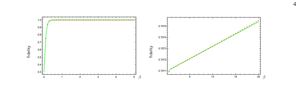
- The method's dependence on the spectral gap $\Delta$ mirrors that of other ground-state algorithms, suggesting that near-degenerate systems (small $\Delta$) will require very large imaginary times $\beta^*$, as the numerical example with $B=0.1$ illustrates.
- A natural extension is to apply the same state-based simulation idea to other nonunitary processes, such as thermal (finite-temperature) state preparation, where the fixed point is the Gibbs state rather than the ground state.
Editorial analysis
A structured set of objections, weighed in public.
Referee Report
Summary. The paper proposes a fully quantum method to simulate imaginary-time evolution using the state-based quantum simulation (SBQS) framework. The Hamiltonian is decomposed into a sum of density-matrix resource states, and the evolution e^{-βH} is approximated by a Trotter-Suzuki product of terms e^{-δ_i ρ_i}. Each term is implemented by preparing an ancilla in a superposition state, applying controlled-SWAP gates between the resource state and the simulator, and postselecting on a measurement outcome. The authors provide error bounds, a probability analysis, and a numerical example for a transverse-field Ising model. The central claim is that the protocol generates the imaginary-time-evolved state to accuracy ε using a number of steps that is inversely proportional to ε and quadratic in the number of resource states.
Significance. If the claims were fully substantiated, the work would offer a conceptually interesting alternative to existing imaginary-time evolution algorithms, removing the need for classical optimization or tomography. The core construction (controlled-SWAP plus postselection on an ancilla) is clean, and the explicit error analysis, including a Trotter-Suzuki bound, is a strength. The worked example on the Ising model provides a useful illustration. However, the paper's central claim is weakened considerably by the exponentially small success probability of the postselected protocol, which is not addressed by any boosting procedure. The mixed-resource-state gap in the derivation is a secondary but real issue. As it stands, the algorithm is best described as a postselected simulation with exponential overhead, not an efficient bounded-error simulation.
major comments (3)
- [§Probability, Eqs. (19)–(20)] The success probability of the protocol is exponentially small, and the analysis gives only an upper bound, so the claim in the Conclusion that the protocol generates the desired imaginary-time evolution 'within a given accuracy' is unsupported in the standard bounded-error sense. From Eq. (12), each step has success probability p_i = Tr[e^{-δ_i ρ_i} σ_{i-1} e^{-δ_i ρ_i}]/2 ≤ 1/2, so after Nℓ steps the total probability is at most 2^{-Nℓ}. Since N* in Eq. (18) grows as (1/(εΔ²)) log²(1/ε), this probability is exponentially small in 1/(εΔ²). Equation (20) states Prob(D ≤ ε) ≤ p*, which is the opposite of what a bounded-error algorithm needs; one requires a lower bound on the success probability. The median-lemma remark on page 4 concedes that the per-step probability is not above 1/2, so the standard repetition-based boosting does not apply, and no amplitude amplification or reset scheme is provided. Without a way to boost the success probability to a constant (or at least to 1/poly), the algorithm's runtime is dominated by an exponential number of repetitions, contradicting the efficiency claimed in the Conclusion.
- [§SBQS of imaginary-time evolution, Eq. (9)] The derivation of the central simulation step assumes pure resource states, whereas the method is stated for general density-matrix decompositions in Eq. (4). The expression (|0⟩|σ0⟩ − δ₁|1⟩ρ₁|σ0⟩)(h.c.) is not the actual post-trace state when ρ₁ is mixed; the reduced state on control and simulator is not rank-one and contains, for example, a δ²|1⟩⟨1| ⊗ ρ₁ term. The first-order postselected term σ − δ{ρ,σ} in Eq. (10) does survive for mixed ρ, so the issue is patchable, but the paper should either restrict the resource states to pure states, justify the general case with a direct derivation, or explicitly state that the derivation is only to first order for mixed ρ.
- [§Conclusion] The runtime statement 'The runtime ... is inversely proportional to simulation error and depends quadratically on the number of necessary resource systems' omits the exponential dependence on N from the success probability. Even with the second strategy's improved per-term probability (ℓ+1)^{-N} in Eq. (23), the expected number of repetitions to obtain one success is exponential in N, and N itself is ∝ 1/(εΔ²) from Eq. (18). Thus the total resource cost is exponential in the inverse error, not just inversely proportional to ε. The conclusion should be revised to state the postselected nature of the protocol and its exponential overhead, or the algorithm must be augmented with a proven boosting procedure.
minor comments (5)
- [Eq. (10)] In the line after Eq. (10), the expression '(I−δ_i ρ_i)σ1(I−δ_i ρ_i)' should refer to σ0 on the right-hand side; as written, σ1 appears on both sides of the approximation.
- [Fig. 2] The label 'n=1000' in the right panel is undefined; specify whether n denotes the number of Trotter steps N or some other parameter.
- [Eq. (6)] The Trotter error is denoted ε_ts in the text and ε in Eq. (7); use a single notation for clarity.
- [Eq. (16)] The factor d in the denominator of Eq. (16) is not derived in the main text; the Supplemental Material gives a tighter bound without d, so either derive Eq. (16) or align it with the SM bound.
- [Second strategy, §Probability] The phrase 'N/2^{ℓ+1}' near the end of the Probability section is likely a typo; the success probability for one step with local measurements is Tr[...]/2^ℓ, and the improvement is to Tr[...]/(ℓ+1).
Circularity Check
No significant circularity; the controlled-SWAP imaginary-time derivation is self-contained and the only overlapping-author citation is not load-bearing.
full rationale
The derivation is self-contained. The one-step map in Eqs. (8)-(10) is obtained by explicit calculation: preparing |ψ_δ1⟩, applying the controlled-SWAP U_cs1, tracing out the resource register, and postselecting |+⟩ gives (σ0−δ1{ρ1,σ0})/2, which matches (I−δ1ρ1)σ0(I−δ1ρ1)/2 up to O(δ1^2); this is a direct computation rather than the target result being assumed. The Trotter decomposition in Eq. (6) follows algebraically from H=Σh_iρ_i with δ_i=βh_i/N, and the coefficients h_i are fixed by the known Hamiltonian, not fitted to any output. The error bound in Eq. (15) and the fidelity bound in Eq. (16) are standard norm and spectral-gap estimates with no fitted parameters. The overlapping-author citation [36] supplies the SBQS decomposition framework, but no correctness statement in the proof is imported from it; the postselected evolution is derived in the present paper. The pure-resource-state assumption in Eq. (9) and the exponentially small success probability in Eq. (19) are correctness gaps that should be weighed separately; they do not make the claimed simulation equivalent to its inputs by construction. No fitted parameter is renamed as a prediction, and no known result is merely relabeled.
Assumptions & free parameters
assumptions (4)
- standard math Trotter-Suzuki product formula applies to the nonunitary semigroup generated by the operators beta h_i rho_i.
- standard math Density matrix exponentiation via controlled-SWAP produces the operation e^{-delta rho} on the simulator state.
- ad hoc to paper Resource states rho_i are pure states.
- domain assumption The Hamiltonian can be shifted to be positive and decomposed into resource states with positive coefficients.
Cite this review
Pith. "Pith review of State-Based Quantum Simulation of Imaginary-Time Evolution." pith.science (2026). https://pith.science/paper/CJTTNC6V
@misc{pith2026250612381,
  author       = {Pith},
  title        = {Pith review of: State-Based Quantum Simulation of Imaginary-Time Evolution},
  year         = {2026},
  howpublished = {\url{https://pith.science/paper/CJTTNC6V}},
  note         = {Machine review of arXiv:2506.12381}
}
read the original abstract
Imaginary time evolution is a powerful technique for computing the ground state of quantum Hamiltonians, where the convergence to ground state in asymptotic imaginary time is guaranteed. However, implementing this method on quantum computers is challenging due to its nonunitary nature. Here, we propose a fully quantum approach for simulation of imaginary time evolutions which eliminates the need for intermediate classical computation or state tomography. Our method leverages the recently introduced state-based quantum simulation technique, in which using quantum states besides quantum gates allows to simulate a broader class of evolutions beyond the natural quantum dynamics. Specifically, we demonstrate how by using a set of quantum states and by applying only controlled-SWAP gates and measurements, one can simulate the nonunitary imaginary time evolution. We illustrate our results in an example.
Figures

Reference graph
Works this paper leans on
-
[1]
N. Schuch and F. Verstraete, Computational complexity of in- teractingelectronsandfundamentallimitationsofdensityfunc- tional theory, Nature Phys.5, 732 (2009)
work page 2009
-
[2]
To simulate the imaginary- time evolution of this Hamiltonian, according to the decom- position (6), we need to simulate three different types of terms, i.e.,𝑈𝑖,𝑖+1 =𝑒 𝛿1𝜚𝑖,𝑖+1⊗I ¯𝑖,𝑖+1,𝑈 𝑋𝑖 =𝑒 𝛿2𝜚𝑋𝑖⊗I ¯𝑖, and 𝑈𝑍𝑖 =𝑒 𝛿3𝜚𝑍𝑖⊗I ¯𝑖, with𝛿 1 =𝛿 2 =4𝐽𝛽/𝑁and𝛿 3 =2𝐵𝛽/𝑁, such that𝑒− 𝛽 𝑁𝐻≈ Î𝑚 𝑖=−𝑚𝑈𝑍𝑖𝑈𝑋𝑖𝑈𝑖,𝑖+1. To make sure that initial state of the simulator has a ...
-
[3]
P.Deglmann,A.Schäfer,andC.Lennartz,Applicationofquan- tum calculations in the chemical industry—an overview, Int. J. Quantum Chem.115, 107 (2015)
work page 2015
-
[4]
C.UmeanoandO.Kyriienko,Groundstate-basedquantumfea- ture maps, arXiv:2404.07174
-
[5]
P. S. Emani, J. Warrell, A. Anticevic, S. Bekiranov, M. Gandal, M. J. McConnell, G. Sapiro, A. Aspuru-Guzik, J. T. Baker, M. Bastiani, J.D.Murray, S.N.Sotiropoulos, J.Taylor, G.Senthil, T. Lehner, M. B. Gerstein, and A. W. Harrow, Quantum com- puting at the frontiers of biological sciences, Nature Methods 18, 701 (2021)
work page 2021
-
[6]
W. M. C. Foulkes, L. Mitas, R. J. Needs, and G. Rajagopal, Quantum Monte Carlo simulations of solids, Rev. Mod. Phys. 73, 33 (2001)
work page 2001
-
[7]
N. Giordano and H. Nakanishi,Computational Physics (Prentice-Hall, Upper Saddle River, NJ, 2006)
work page 2006
-
[8]
G. C. Wick, Properties of Bethe-Salpeter wave functions, Phys. Rev.96, 1124 (1954)
work page 1954
Show all 52 references
-
[9]
M.G.Mustafa,AnIntroductiontothermalfieldtheoryandsome of its application, Eur. Phys. J. ST2321369 (2023)
2023
-
[10]
A.Das,FiniteTemperatureFieldTheory(WorldScientific,Sin- gapore, 2023)
2023
-
[11]
Zwolak and G
M. Zwolak and G. Vidal, Mixed-State Dynamics in One- Dimensional Quantum Lattice Systems: A Time-Dependent Superoperator Renormalization Algorithm, Phys. Rev. Lett.93, 207205 (2004)
2004
-
[12]
Verstraete, J
F. Verstraete, J. J. García-Ripoll, and J. I. Cirac, Matrix Prod- uct Density Operators: Simulation of Finite-Temperature and Dissipative Systems, Phys. Rev. Lett.93, 207204 (2004)
2004
-
[13]
F. A. Wolf, A. Go, I. P. McCulloch, A. J. Millis, and U. Scholl- wöck, Imaginary-time matrix product state impurity solver for dynamical mean-field theory, Phys. Rev. X5, 041032 (2015)
2015
-
[14]
Kumar and C
S. Kumar and C. M. Wilmott, Generalising quantum imaginary time evolution to solve linear partial differential equations. Sci. Rep.14, 20156 (2024)
2024
-
[15]
Oliveira and B
R. Oliveira and B. M. Terhal, The complexity of quantum spin systems on a two-dimensional square lattice, Quant. Inf. Com- put.8, 0900 (2008)
2008
-
[16]
Comput.,35,1070 (2006)
J.Kempe,A.Kitaev,andO.Regev,Thecomplexityofthelocal Hamiltonian problem, SIAM J. Comput.,35,1070 (2006)
2006
-
[17]
Aharonov, D
D. Aharonov, D. Gottesman, S. Irani, and J. Kempe, The power of quantum systems on a line, Commun. Math. Phys.287, 41 (2009)
2009
-
[18]
A. Yu. Kitaev, Quantum measurements and the Abelian stabi- lizer problem, arXiv:quant-ph/9511026 (1995)
1995 arXiv
-
[19]
Cleve, A
R. Cleve, A. Ekert, C. Macchiavello, and M. Mosca, Quantum algorithmsrevisited,Proc.Roy.Soc.LondonA454,339(1998)
1998
-
[20]
Lin, A note on quantum phase estimation, arXiv:2304.02241
Y.-T. Lin, A note on quantum phase estimation, arXiv:2304.02241
-
[21]
A.Aspuru-Guzik,A.D.Dutoi,P.J.Love,andM.Head-Gordon, Simulatedquantumcomputationofmolecularenergies,Science 309, 1704 (2005)
2005
-
[22]
L.LinandY.Tong,Heisenberg-limitedground-stateenergyes- timationforearlyfault-tolerantquantumcomputers,PRXQuan- tum,3, 010318 (2022)
2022
-
[23]
Y. Dong, L. Lin, and Y. Tong, Ground-state preparation and energyestimationonearlyfault-tolerantquantumcomputersvia quantum eigenvalue transformation of unitary matrices, PRX Quantum,3, 040305 (2022)
2022
-
[24]
R. D. Somma, Quantum eigenvalue estimation via time series analysis, New. J. Phys.21,123025 (2019)
2019
-
[25]
G.Wang,D.S.Franca,R.Zhang,S.Zhu,andP.Johnson,Quan- tum algorithm for ground state energy estimation using circuit depth with exponentially improved dependence on precision, Quantum8, 1496 (2024)
2024
-
[26]
A. B. Finnila, M. A. Gomez, C. Sebenik, C. Stenson, and J. D. Doll, Quantum annealing: a new method for minimizing multidimensionalfunctions,Chem.Phys.Lett.219,343(1994)
1994
-
[27]
T.KadowakiandH.Nishimori,Quantumannealinginthetrans- verse Ising model, Phys. Rev. E58, 5355 (1998)
1998
-
[28]
Farhi, J
E. Farhi, J. Goldstone, S. Gutmann, and M. Sipser, Quantum computation by adiabatic evolution, arXiv:quant-ph/0001106
-
[29]
E.Farhi,J.Goldstone,andS.Gutmann,Aquantumapproximate optimization algorithm, arXiv:1411.4028
-
[30]
Peruzzo, J
A. Peruzzo, J. McClean, P. Shadbolt, M.-H. Yung, X.-Q. Zhou, P. J. Love, A. Aspuru-Guzik, and J. L. O’Brien, A variational eigenvalue solver on a photonic quantum processor, Nature Commun.5, 4213 (2014)
2014
-
[31]
Kandala, A
A. Kandala, A. Mezzacapo, K. Temme, M. Takita, M. Brink, J. M. Chow, and J. M. Gambetta, Hardware-efficient variational quantumeigensolverforsmallmoleculesandquantummagnets, Nature549, 242 (2017)
2017
-
[32]
X. Yuan, S. Endo, Q. Zhao, Y. Li, and S. C. Benjamin, Theory of variational quantum simulation, Quantum3, 191 (2019)
2019
-
[33]
J.Stokes, J.Izaac, N.Killoran, andG.Carleo, Quantumnatural gradient, Quantum4, 269 (2020). 6
2020
-
[34]
McArdle, T
S. McArdle, T. Jones, S. Endo, Y. Li, S. C. Benjamin, and X. Yuan, Variational ansatz-based quantum simulation of imagi- nary time evolution, npj Quantum Info.75, 5 (2019)
2019
-
[35]
Motta, C
M. Motta, C. Sun, A. T. K. Tan, M. J. O’Rourke, E. Ye, A. J. Minnich, F. G. S. L. Brandão, and G. K.-L. Chan, Determining eigenstates and thermal states on a quantum computer using quantumimaginarytimeevolution,NaturePhys.16,205(2020)
2020
-
[36]
Nishi, T
H. Nishi, T. Kosugi, and Y. Matsushita, Implementation of quantum imaginary-time evolution method on NISQ devices by introducing nonlocal approximation, npj Quantum Info.7, 85 (2021)
2021
-
[37]
Alipour, A
S. Alipour, A. T. Rezakhani, A. Tavanfar, K. Mølmer, T. Ala- Nissila, State-based quantum simulation: Releasing power of quantum states and copies, arXiv:2505.13901
-
[38]
M. A. Nielsen and I. L. Chuang,Quantum Computation and Quantum Information(Cambridge University Press, Cam- bridge, 2010)
2010
-
[39]
J.Preskill,Quantumcomputing40yearslater,inFeynmanLec- turesonComputation,editedbyT.Hey(CRCPress,BocaRaton, FL, 2023)
2023
-
[40]
D. S. Abrams and S. Lloyd, Simulation of Many-Body Fermi SystemsonaUniversalQuantumComputer,Phys.Rev.Lett.79, 2586 (1997)
1997
-
[41]
D. S. Abrams and S. Lloyd, Quantum Algorithm Providing ExponentialSpeedIncreaseforFindingEigenvaluesandEigen- vectors, Phys. Rev. Lett.83, 5162 (1999)
1999
-
[42]
K. L. Brown, W. J. Munro, and V. M. Kendon, Using quantum computers for quantum simulation, Entropy12, 2268 (2010)
2010
-
[43]
I. M. Georgescu, S. Ashhab, and F. Nori, Quantum simulation, Rev. Mod. Phys.86, 153 (2014)
2014
-
[44]
Lloyd, M
S. Lloyd, M. Mohseni, and P. Rebentrost, Quantum principal component analysis, Nature Phys.10, 631 (2014)
2014
-
[45]
Kjaergaard, M
M. Kjaergaard, M. E. Schwartz, A. Greene, G. O. Samach, A. Bengtsson, M. O’Keeffe, C. M. McNally, J. Braumüller, D. K. Kim, P. Krantz, M. Marvian, A. Melville, B. M. Niedzielski, Y. Sung, R. Winik, J. Yoder, D. Rosenberg, K. Obenland, S. Lloyd, T. P. Orlando, I. Marvian, S. Gu...
2022
-
[46]
Rivas and S
Á. Rivas and S. F. Huelga,Open Quantum Systems(Springer, Berlin, 2012)
2012
-
[47]
A.M.Childs,Y.Su,M.C.Tran,N.Wiebe,andS.Zhu,Theoryof Trottererrorwithcommutatorscaling,Phys.Rev.X11,011020 (2021)
2021
-
[48]
Ostmeyer, Optimised Trotter decompositions for classical and quantum computing, J
J. Ostmeyer, Optimised Trotter decompositions for classical and quantum computing, J. Phys. A: Math. Theor.56, 285303 (2023)
2023
-
[49]
V. A. Zagrebnov, H. Neidhardt, and T. Ichinose,Trotter-Kato Product Formulæ(Birkhäuser, 2024)
2024
-
[50]
Wiebe, A
N. Wiebe, A. Kapoor, and K. M. Svore, Quantum algorithms for nearest-neighbor methods for supervised and unsupervised learning, arXiv:1401.2142
-
[51]
A.Tavanfar,A.Parvizi,M.Pezzutto,Unitaryevolutionssourced by interacting quantum memories: Closed quantum systems directingthemselvesusingtheirstatehistories,Quantum7,1007 (2023)
2023
-
[52]
Tavanfar, S
A. Tavanfar, S. Alipour, and A. T. Rezakhani, Does quantum mechanics breed larger, more intricate quantum theories? The caseforexperience-centricquantumtheoryandtheinteractome of quantum theories, Universe11, 162 (2025). 7 Supplemental Material Error of multiplication of erron...
2025
Reviewed August 7, 2026 · model on record in the stance chip above.
Discussion (0). Sign in to comment.