REVIEW 4 major objections 5 minor 42 references
PINNs Algorithmic Framework for Simulation of Nonlinear Burgers' Type Models
T0 review · 4 major / 5 minor · reviewed 2026-08-07 · deepseek-v4-flash
Pith's one-line read The paper claims that a physics-informed neural network trained on PDE residuals, initial data, and boundary data accurately simulates 1D and 2D nonlinear Burgers-type models and, on the paper's comparison tables, beats four classical…
desk verdict Standard PINN applied to smooth Burgers benchmarks, but the headline accuracy comparisons are unreproducible because the printed residual does not match Example 2 and no code, training details, or selected architecture are given. read the letter →
The pith
A machine-rendered reading of the paper's core claim, the machinery that carries it, and where it could break.
The reading
What carries the argument
The load-bearing object is the composite physics-informed loss $L_{\mathrm{total}} = L_{\mathrm{PDE}} + 10 L_{\mathrm{IC}} + 10 L_{\mathrm{BC}}$, where $L_{\mathrm{PDE}}$ is the mean squared residual of the Burgers-type system evaluated with automatic differentiation at collocation points, and $L_{\mathrm{IC}}$ and $L_{\mathrm{BC}}$ are mean squared mismatches of initial and boundary conditions. The trial solution is a fully connected feed-forward network with tanh activations that maps space-time coordinates to the solution components; because derivatives come from automatic differentiation, no mesh or discretized grid appears in the algorithm. The paper sweeps depth $L \in \{3,4,5,6,7\}$ and width $H \in \{20,30,40,50,60\}$ to select an architecture, then trains with the Adam optimizer at learning rate $10^{-3}$.
What would settle it
Re-running the paper's Example 2 with the stated loss weights and Adam settings while recording the actual architecture size and training point counts would settle whether the printed $L^\infty$ and $L^2$ errors for both solution components reproduce across random seeds; if the rerun error varies widely or fails to stay below the four baseline values, the claimed superiority would not hold up.
Extended reading notes
Core claim
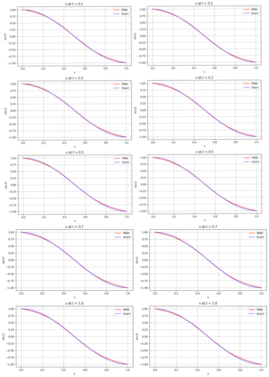
The central claim is that a fully connected feed-forward network with tanh activations, taking space-time coordinates as input and returning the solution components as output, can approximate the exact solutions of the coupled Burgers systems when trained to minimize the composite loss $L_{\mathrm{total}} = L_{\mathrm{PDE}} + 10 L_{\mathrm{IC}} + 10 L_{\mathrm{BC}}$. The PDE residual is evaluated by automatic differentiation, so no spatial discretization appears in the method. The paper's strongest quantitative assertion is in its second example, where the reported $L^\infty$ and $L^2$ errors for the first solution component are lower at the tabulated times than the errors it attributes to the four cited baseline methods; the conclusion states that PINN offers better and more effective results than those references. The paper also reports stable solutions at Reynolds number $10^6$, a regime where conventional mesh-based schemes often require stabilization.
Load-bearing premise
The superiority claim rests on the error tables being reproducible from the setup as described and on the cited comparison errors being computed under equivalent conditions, but the paper does not report the chosen depth and width, the number of collocation, initial, and boundary points, the number of training epochs, the random seed, or the stopping criterion.
Editorial extensions
If this is right
- If the central claim is correct, nonlinear coupled Burgers problems can be simulated without generating a mesh, which lowers the setup cost for problems on irregular or high-dimensional domains.
- The reported stability at Reynolds number $10^6$ suggests the same network formulation could handle advection-dominated flows where classical schemes need added stabilization.
- Since one architecture and loss recipe covers 1D coupled, 2D scalar, and 2D coupled models, the result implies the method transfers across PDE systems with minimal reformulation.
- If the comparison tables are accepted, PINNs become a practical default benchmark solver for nonlinear Burgers-type equations and similar convection-diffusion systems.
- Because the trial solution is fully differentiable, the trained representation can supply gradients needed for downstream sensitivity analysis or optimization without extra discretization.
Reading between the lines
- Beyond the paper, the same composite loss could be applied to other coupled parabolic systems such as reaction-diffusion or shallow-water equations, since the machinery is problem-agnostic apart from the residual definition.
- Beyond the paper, the fixed weighting of the initial and boundary loss terms is a knob worth tuning adaptively; loss reweighting could reduce the boundary-adjacent discrepancies the paper itself observes in its first example.
- Beyond the paper, the claimed advantage over the cited baselines could be tested directly by re-implementing those methods on identical grids and norms instead of importing published error numbers.
Editorial analysis
A structured set of objections, weighed in public.
Referee Report
Summary. The paper proposes a physics-informed neural network (PINN) framework for simulating nonlinear Burgers-type equations, and demonstrates it on five test problems: 1D coupled, 2D single, and 2D coupled Burgers models. The reported results, especially for Example 2, are compared against existing methods (Bak, Ahmad, Khater, Rashid) in terms of L2 and L-infinity errors, and the conclusion claims that PINN offers better and more effective results than those references. The manuscript also describes the network architecture, loss function, and training procedure, though without providing the numerical details needed for reproduction.
Significance. If the reported results were reproducible and the comparisons fair, the paper would provide a useful benchmark for applying PINNs to coupled Burgers-type equations, particularly in the high-Reynolds-number regime and in 2D. The exact solutions quoted for Examples 1–3 appear to satisfy the stated equations, which is a strength. However, the manuscript as written does not establish its central quantitative claims: the printed loss function and initial condition in Section 4 match only Example 3, not the Example 2 source of the headline comparison; the training configuration is under-specified; and the reported tables do not uniformly support the claimed superiority over the cited baselines. These issues undermine the verifiability of the error tables and the validity of conclusion (iii).
major comments (4)
- [§4 vs §5, Example 2] Section 4 defines the PDE residuals as f_u = u_t − εu_xx + 2u u_x − (uv)_x and the initial condition as u(x,0)=v(x,0)=cos(πx). This matches only Example 3, whose exact solution is e^{−ε π² t} cos(πx). Example 2, the only example with a comparison to prior methods, uses u_t − u_xx − 2u u_x + 0.1(uv)_x = 0 with tanh-type initial profiles. Substituting the Example 2 exact solution into the Section 4 residual gives a nonzero value (approximately −2.7e−5 at t=0.5, x=0), so the printed loss cannot be the loss that produced Tables 5.2 and 5.3. The paper never states the residual actually minimized for Examples 1, 2, 4, or 5.
- [§3.1, §5 Algorithm step 4] The manuscript does not provide the information needed to reproduce the numerical results. Section 3.1 reports a hyperparameter sweep over L ∈ {3,4,5,6,7} and H ∈ {20,30,40,50,60} but never states the selected depth and width. Algorithm Step 4 says 'For E epochs' but E is never defined. The paper does not report the number of collocation, initial-condition, or boundary-condition points, the random seed, or any learning-rate schedule beyond the generic Adam defaults. The Data Availability statement says no data will be made available, and no code is referenced. Consequently, the error values in Tables 5.1–5.3 and the figures cannot be independently verified.
- [Tables 5.2 and 5.3, §6 (iii)] The claim that 'PINN demonstrates significantly lower L∞ and L2 errors for both u and v compared to existing methods' is contradicted by the tables themselves. At t=0.5, Ahmad et al. [1] reports L∞ = 2.1840e−4 for u and 2.5169e−4 for v, while the PINN errors are 3.2962e−4 and 6.4322e−4, respectively. Thus the PINN is worse than at least one baseline at the earliest reported time. In addition, Table 5.3 labels the PINN columns as 'error_u' although the table is for v, and several entries for Khater and Rashid are missing. The comparison also gives no information about the grids, norms, or stopping criteria used in the baseline papers, so the conclusion of superiority is not established.
- [§5, Examples 4 and 5] The abstract and Section 6 state that the method is validated through L2 and L-infinity error norms, but Examples 4 and 5 (2D single and 2D coupled Burgers) are presented only through figures (Figs. 5.6–5.8), with no error tables or convergence measurements. Without quantitative error metrics for these two examples, the claim of rigorous validation for higher-dimensional cases is not supported.
minor comments (5)
- [Abstract] The phrase 'competitive performance in terms of inaccuracy' should be 'accuracy'; 'inaccuracy' is presumably a typo.
- [§5, opening paragraph] The text says the method is applied to 'three different example' but the paper presents five examples; the count should be corrected.
- [§5, Example 2 discussion] The sentence 'Errors shown in Table 5.2 of the problem are an order of magnitude smaller than in problems 1–2' should refer to 'Example 1', since this is Example 2.
- [Eq. (4.2)] The symbol ε is used both for the PDE viscosity coefficient and for the Adam optimizer's small constant in Eq. (4.2); this notational collision could confuse readers.
- [§2, Eq. (2.3)] The notation u·∇u is ambiguous in the 1D setting where u is a scalar; the examples later use u u_x, so the general formulation should clarify the intended interpretation.
Circularity Check
No circularity: error tables are independent benchmarks against analytic solutions; self-citations and hyperparameter tuning are not load-bearing.
full rationale
The paper's only quantitative claims are the error norms in Tables 5.1, 5.2, and 5.3, which are computed by comparing a trained network to closed-form analytic solutions. These solutions are independent of the network's training data except for the standard soft initial- and boundary-condition penalties. The PINN loss in Section 4 (Eq. 4.1) is a standard residual-minimization objective, and no parameter is fitted to the reported error values themselves. The hyperparameter sweep in Section 3.1 selects depth and width by validation error; that is ordinary model selection, and the paper does not state that the validation set coincides with the reported test evaluation points, so no statistically forced 'prediction' is established. The self-citations in the introduction (refs. [16, 17, 18, 20]) and the use of [31] for the Example 1 exact solution are contextual and do not carry the derivation of the PINN method or its comparative claims. The serious weaknesses here—that the Section 4 residual and initial condition match only Example 3 and not Example 2 (the source of the headline comparison), the undisclosed training configuration, and the Data Availability statement saying no data will be made available—are reproducibility and correctness concerns, not circular reasoning. No step in the claimed derivation chain reduces to its own input by construction.
Assumptions & free parameters
free parameters (4)
- Network depth L =
not reported (search range 3 to 7)
- Network width H =
not reported (search range 20 to 60)
- Loss weights lambda_IC and lambda_BC =
10
- Training sample counts (collocation, IC, BC points) =
not reported
assumptions (4)
- domain assumption The quoted exact and manufactured solutions solve the stated PDEs and provide valid initial and boundary data.
- domain assumption A fully connected tanh network trained on sampled residual, initial condition, and boundary condition losses approximates the PDE solution over the entire space-time domain.
- ad hoc to paper The loss definition in Section 4 corresponds to the problems actually solved in Section 5.
- domain assumption The literature baseline errors are comparable in norm, grid, and implementation.
Cite this review
Pith. "Pith review of PINNs Algorithmic Framework for Simulation of Nonlinear Burgers' Type Models." pith.science (2026). https://pith.science/paper/AOMIIZR2
@misc{pith2026250612922,
  author       = {Pith},
  title        = {Pith review of: PINNs Algorithmic Framework for Simulation of Nonlinear Burgers' Type Models},
  year         = {2026},
  howpublished = {\url{https://pith.science/paper/AOMIIZR2}},
  note         = {Machine review of arXiv:2506.12922}
}
read the original abstract
In this work, a physics-informed neural networks (PINNs) based algorithm is used for simulation of nonlinear 1D and 2D Burgers' type models. This scheme relies on a neural network built to approximate the problem solution and use a trial function that meets the initial data and boundary criteria. First of all, a brief mathematical formulation of the problem and the structure of PINNs, including the neural network architecture, loss construction, and training methodology is described. Finally, the algorithm is demonstrated with five test problems involving variations of the 1D coupled, 2D single and 2D coupled Burgers' models. We compare the PINN-based solutions with exact results to assess accuracy and convergence of the developed algorithm. The results demonstrate that PINNs may faithfully replicate nonlinear PDE solutions and offer competitive performance in terms of inaccuracy and flexibility. This work demonstrates the potential of PINNs as a reliable approach to solving complex time-dependent PDEs.
Figures


Figures from the paper (6 more)



Reference graph
Works this paper leans on
- [34]
- [1]
-
[2]
M. S. Alnæs, J. Hake, R. C. Kirby, H. P. Langtangen, A. Logg, and G. N. Wells. The fenics manual.FEniCS Project, version October 31st, 36, 2011
work page 2011
-
[3]
S. Bak, P. Kim, and D. Kim. A semi-lagrangian approach for numerical simulation of coupled burgers’ equations.Communications in Nonlinear Science and Numerical Simulation, 69:31–44, 2019
work page 2019
-
[4]
A. G. Baydin, B. A. Pearlmutter, A. A. Radul, and J. M. Siskind. Automatic differentiation in machine learning: a survey.Journal of machine learning research, 18(153):1–43, 2018
work page 2018
- [5]
-
[6]
H.-J. Bungartz and M. Griebel. Sparse grids.Acta numerica, 13:147–269, 2004
work page 2004
-
[7]
J. M. Burgers.The nonlinear diffusion equation: asymptotic solutions and statistical problems. Springer Science & Business Media, 2013
work page 2013
Show all 42 references
-
[8]
F. Chen, D. Sondak, P. Protopapas, M. Mattheakis, S. Liu, D. Agarwal, and M. Di Giovanni. Neurodiffeq: A python package for solving differential equations with neural networks.Journal of Open Source Software, 5(46):1931, 2020. 16
1931
-
[9]
J. Ding, C. Liu, Y. Zheng, Y. Zhang, Z. Yu, R. Li, H. Chen, J. Piao, H. Wang, J. Liu, et al. Ar- tificial intelligence for complex network: Potential, methodology and application.arXiv preprint arXiv:2402.16887, 2024
2024 arXiv
-
[10]
Egger, U
H. Egger, U. Rüde, and B. Wohlmuth. Energy-corrected finite element methods for corner sin- gularities.SIAM Journal on Numerical Analysis, 52(1):171–193, 2014
2014
-
[11]
Hennigh, S
O. Hennigh, S. Narasimhan, M. A. Nabian, A. Subramaniam, K. Tangsali, Z. Fang, M. Riet- mann, W. Byeon, and S. Choudhry. Nvidia simnet™: An ai-accelerated multi-physics simulation framework. InInternational conference on computational science, pages 447–461. Springer, 2021
2021
-
[12]
A. J. Hussein and H. A. Kashkool. Weak galerkin finite element method for solving one- dimensional coupled burgers’ equations.Journal of Applied Mathematics and Computing, 63(1):265–293, 2020
2020
-
[13]
Number44.Cambridge university press, 2009
A.Iserles.A first course in the numerical analysis of differential equations. Number44.Cambridge university press, 2009
2009
-
[14]
A. D. Jagtap and G. E. Karniadakis. Extended physics-informed neural networks (xpinns): A generalized space-time domain decomposition based deep learning framework for nonlinear partial differential equations.Communications in Computational Physics, 28(5), 2020
2020
-
[15]
A. D. Jagtap, E. Kharazmi, and G. E. Karniadakis. Conservative physics-informed neural net- works on discrete domains for conservation laws: Applications to forward and inverse problems. Computer Methods in Applied Mechanics and Engineering, 365:113028, 2020
2020
-
[16]
R. Jiwari. A haar wavelet quasilinearization approach for numerical simulation of burgers’ equa- tion.Computer Physics Communications, 183(11):2413–2423, 2012
2012
-
[17]
R. Jiwari. A hybrid numerical scheme for the numerical solution of the burgers’ equation.Com- puter Physics Communications, 188:59–67, 2015
2015
-
[18]
R. Jiwari. Local radial basis function-finite difference based algorithms for singularly perturbed burgers’ model.Mathematics and Computers in Simulation, 198:106–126, 2022
2022
-
[19]
Jiwari and N
R. Jiwari and N. Kumar. Analysis and simulation of korteweg-de vries-rosenau-regularised long- wave model via galerkin finite element method.Computers & Mathematics with Applications, 135:134–148, 2023
2023
-
[20]
Jiwari, S
R. Jiwari, S. Kumar, and R. Mittal. Meshfree algorithms based on radial basis functions for numerical simulation and to capture shocks behavior of burgers’ type problems.Engineering Computations, 36(4):1142–1168, 2019
2019
-
[21]
Jiwari and S
R. Jiwari and S. Singh. Finite element method for the numerical simulation of modified poisson- nernst-planck/navier-stokes model.arXiv preprint arXiv:2409.08746, 2024
2024
-
[22]
G. E. Karniadakis, I. G. Kevrekidis, L. Lu, P. Perdikaris, S. Wang, and L. Yang. Physics-informed machine learning.Nature Reviews Physics, 3(6):422–440, 2021
2021
-
[23]
Kharazmi, Z
E. Kharazmi, Z. Zhang, and G. E. Karniadakis. Variational physics-informed neural networks for solving partial differential equations.arXiv preprint arXiv:1912.00873, 2019. 17
1912 arXiv
-
[24]
Khater, R
A. Khater, R. Temsah, and M. Hassan. A chebyshev spectral collocation method for solving burgers’-typeequations.Journal of computational and applied mathematics, 222(2):333–350, 2008
2008
-
[25]
D. P. Kingma and J. Ba. Adam: A method for stochastic optimization.arXiv preprint arXiv:1412.6980, 2014
2014 arXiv
-
[26]
Kovacs, L
A. Kovacs, L. Exl, A. Kornell, J. Fischbacher, M. Hovorka, M. Gusenbauer, L. Breth, H. Oezelt, M. Yano, N. Sakuma, et al. Conditional physics informed neural networks.Communications in Nonlinear Science and Numerical Simulation, 104:106041, 2022
2022
-
[27]
Kumar, A
N. Kumar, A. Singh, R. Jiwari, and J. Yuan. Error estimates with polynomial growth o (ε- 1) for the hho method on polygonal meshes of the allen-cahn model.Applied Numerical Mathematics, 211:78–102, 2025
2025
-
[28]
W. Li, M. Z. Bazant, and J. Zhu. A physics-guided neural network framework for elastic plates: Comparison of governing equations-based and energy-based approaches.Computer Methods in Applied Mechanics and Engineering, 383:113933, 2021
2021
-
[29]
L. Lu, X. Meng, Z. Mao, and G. E. Karniadakis. Deepxde: A deep learning library for solving differential equations.SIAM review, 63(1):208–228, 2021
2021
-
[30]
Z. Mao, A. D. Jagtap, and G. E. Karniadakis. Physics-informed neural networks for high-speed flows.Computer Methods in Applied Mechanics and Engineering, 360:112789, 2020
2020
-
[31]
Mittal and R
R. Mittal and R. Jiwari. Differential quadrature method for numerical solution of coupled viscous burgers’ equations.International Journal for Computational Methods in Engineering Science and Mechanics, 13(2):88–92, 2012
2012
-
[32]
Mittal and A
R. Mittal and A. Tripathi. A collocation method for numerical solutions of coupled burgers’ equations.International Journal for computational methods in engineering science and mechanics, 15(5):457–471, 2014
2014
-
[33]
Moseley, A
B. Moseley, A. Markham, and T. Nissen-Meyer. Finite basis physics-informed neural networks (fbpinns): a scalable domain decomposition approach for solving differential equations.Advances in Computational Mathematics, 49(4):62, 2023
2023
-
[35]
Rashid and A
A. Rashid and A. I. B. M. Ismail. A fourier pseudospectral method for solving coupled viscous burgers equations.Computational Methods in Applied Mathematics, 9(4):412–420, 2009
2009
-
[36]
Sheng and T
Y. Sheng and T. Zhang. The finite volume method for two-dimensional burgers’ equation.Per- sonal and Ubiquitous Computing, 22(5):1133–1139, 2018
2018
-
[37]
Singh, H
A. Singh, H. M. Cheng, N. Kumar, and R. Jiwari. A high order numerical method for analysis and simulation of 2d semilinear sobolev model on polygonal meshes.Mathematics and Computers in Simulation, 227:241–262, 2025. 18
2025
-
[38]
J. D. Smith, Z. E. Ross, K. Azizzadenesheli, and J. B. Muir. Hyposvi: Hypocentre inversion with stein variational inference and physics informed neural networks.Geophysical Journal Interna- tional, 228(1):698–710, 2022
2022
-
[39]
Thanasutives, M
P. Thanasutives, M. Numao, and K.-i. Fukui. Adversarial multi-task learning enhanced physics- informed neural networks for solving partial differential equations. In2021 International Joint Conference on Neural Networks (IJCNN), pages 1–9. IEEE, 2021
2021
-
[40]
A.-M. Wazwaz. Multiple-front solutions for the burgers equation and the coupled burgers equa- tions.Applied mathematics and computation, 190(2):1198–1206, 2007
2007
-
[41]
Wojtowytsch and E
S. Wojtowytsch and E. Weinan. Can shallow neural networks beat the curse of dimensionality? a mean field training perspective.IEEE Transactions on Artificial Intelligence, 1(2):121–129, 2020
2020
-
[42]
Adeeplearningframeworkforsolvingforwardandinverseproblems of power-law fluids.Physics of Fluids, 35(9), 2023
R.Zhai, D.Yin, andG.Pang. Adeeplearningframeworkforsolvingforwardandinverseproblems of power-law fluids.Physics of Fluids, 35(9), 2023. 19
2023
Reviewed August 7, 2026 · model on record in the stance chip above.
Discussion (0). Continue with ORCID to comment.