REVIEW 3 major objections 5 minor 1 cited by
Fast Convergence for High-Order ODE Solvers in Diffusion Probabilistic Models
T0 review · 3 major / 5 minor · reviewed 2026-08-07 · deepseek-v4-flash
Pith's one-line read The paper proves that deterministic samplers for diffusion probabilistic models—probability flow ODEs solved with p-th order (exponential) Runge-Kutta schemes—converge in total variation with polynomial dependence on dimension, provided…
desk verdict A real advance in deterministic diffusion sampling theory—C² score smoothness suffices—but the empirical verification of the load-bearing smoothness assumption is not yet rigorous. read the letter →
The pith
A machine-rendered reading of the paper's core claim, the machinery that carries it, and where it could break.
The reading
What carries the argument
The argument is carried by two discrete flows over a single step: the map $\phi_H$ built from the true score with the Runge-Kutta coefficients, the map $\tilde{\phi}_H$ built from the estimated score, and the interpolation $\varphi_s$ between their inverses. The total variation error is split as $I_1 + I_2 + I_3$, where $I_1$ is the initial distribution error, $I_2$ is the score-matching error, and $I_3$ is the discretization error. $I_2$ is controlled by pushing the reference density through the interpolation and applying the Gagliardo-Nirenberg inequality to trade $L^1$ quantities for the $L^2$ score error, producing the $d^{7/4}\varepsilon_{\mathrm{score}}^{1/2}$ term; $I_3$ is controlled by rewriting the numerical update as an ODE flow and comparing it with the exact flow, producing the $H^p$ term. The load-bearing objects are Assumption 3.5, the uniform derivative bounds $\sup_x|\partial_l s_t^{(j)}(x)| \le \tilde{K}\tau^{-2}$ and $\sup_x|\partial^2_{lk}s_t^{(j)}(x)| \le \tilde{K}\tau^{-3}$, and Lemma 5.6, which establishes that the Runge-Kutta maps are diffeomorphisms and forces the step-size restriction $H_{\max} \le (d\log 2d)^{-1}\tau^3\Delta_{\mathrm{disc}}$. For general forward processes, the enhanced exponential Runge-Kutta schemes of Section 4.2 rewrite the dynamics so that the same propositions apply to the rescaled score.
What would settle it
Use a score network that is not twice differentiable—for instance a ReLU network, which fails Assumption 3.5 because its second derivative does not exist as a bounded function—or compute the actual supremum of $|\partial^2_{lk}s_t^{(j)}(x)|$ on expanding spheres away from the data support; the first test would show that the stated regularity assumption excludes a standard trained model, and the second would settle whether the bound has any footing for the models actually used.
Extended reading notes
Core claim
The central claim is Theorem 3.7, extended to general variance schedules as Theorem 4.2: if the target distribution has compact support, the discrete-time weighted $L^2$ score matching error is at most $\varepsilon_{\mathrm{score}}^2$, all Runge-Kutta evaluation times lie on the score-matching grid, and the learned score has uniformly bounded first and second derivatives (pointwise bounds $\tilde{K}\tau^{-2}$ and $\tilde{K}\tau^{-3}$), then the numerical sampler obeys $TV(\varrho_{T-\tau}, \tilde{\varrho}_{T-\tau}) \le TV(\varrho_0, \tilde{\varrho}_0) + C_{\mathrm{score}}\tau^{-2}T^{3/4}d^{7/4}\varepsilon_{\mathrm{score}}^{1/2} + C_{\mathrm{RK}} T H_{\max}^{p}d^{p+1}\tau^{-\gamma_1}(D+\sqrt{\log d})^{\gamma_2}$, provided $H_{\max} \le (d\log 2d)^{-1}\tau^3\Delta_{\mathrm{disc}}$. Treating the rollout time $T$, the stopping margin $\tau$, and the data diameter $D$ as constants, this is the advertised $O(d^{7/4}\varepsilon_{\mathrm{score}}^{1/2} + d(dH_{\max})^p)$, which yields an iteration complexity of $O(d^{1+1/p}\varepsilon^{-1/p})$ when the score error is negligible. Inside the bound, the score-error term carries the $\varepsilon^{1/2}$ exponent produced by the Gagliardo-Nirenberg interpolation step, and the discretization term carries $p$-th order convergence in the step size; the two errors add rather than compound one another. The authors state the result the way a numerical analyst would: sampling difficulty is set by the score approximation error and the solver order, not by an exponential contraction estimate of the dynamics.
Load-bearing premise
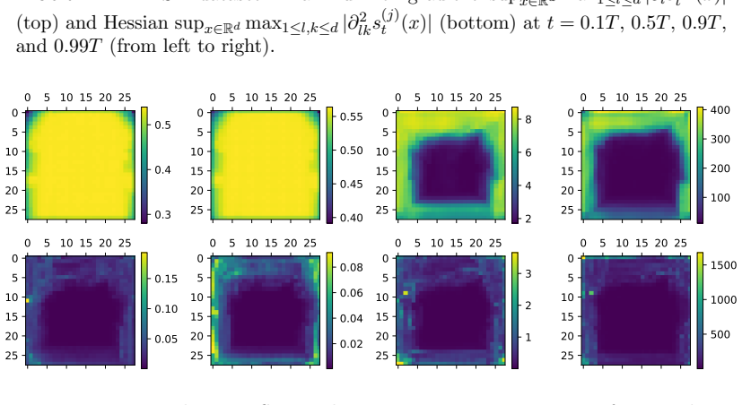
The load-bearing premise is Assumption 3.5, that the learned score function has first and second derivatives uniformly bounded across all of $\mathbb{R}^d$ with the stated $\tau$-scaling; a trained network whose derivatives grow with distance from the data would void the bound, and the paper's empirical check displays pixel-wise maxima over samples rather than computing genuine suprema over $\mathbb{R}^d$.
Editorial extensions
If this is right
- Any $p$-th order (exponential) Runge-Kutta sampler for a probability flow ODE converges in total variation with error $O(d^{7/4}\varepsilon_{\mathrm{score}}^{1/2} + d(dH_{\max})^p)$, so reaching accuracy $\varepsilon$ needs $O(d^{1+1/p}\varepsilon^{-1/p})$ steps when the score error is negligible.
- Only boundedness of the first two derivatives of the estimated score is required, not control of the difference between true and estimated score derivatives as in earlier analyses, and not the higher-order smoothness the authors' own prior work demanded.
- The guarantee covers non-uniform time grids and general forward processes with arbitrary variance schedules, through the enhanced exponential Runge-Kutta schemes whose evaluation times align with the score-matching grid.
- The score error and the discretization error add rather than amplify each other, so improving one source of error does not destabilize the other, and with standard-normal initialization the initial-condition error decays as $e^{-T}\sqrt{d}D$.
Reading between the lines
- The twice-differentiability assumption excludes the cheapest score architectures, since networks with piecewise-linear activations are not $C^2$; a natural stress test is whether the observed convergence rates survive such networks, which would indicate the regularity assumption can be relaxed to an averaged or distributional condition.
- The numerical observation that total variation error scales linearly with $\varepsilon_{\mathrm{score}}$ on Gaussian mixtures suggests the $\varepsilon^{1/2}$ exponent is an artifact of the interpolation step rather than an intrinsic rate; tightening it would likely require an $L^1$-to-$L^2$ stability estimate for the transported density.
- The step-size restriction $H_{\max} \le (d\log 2d)^{-1}\tau^3\Delta_{\mathrm{disc}}$ is demanded only to keep the Runge-Kutta maps invertible, yet the experiments show RK4 working with as few as 8 steps; separating the invertibility condition from the convergence proof could lead to dimension-independent step-size rules.
- The worst-case dimension factors $d^{7/4}$ and $d^{p+1}$ come from moment bounds over the full ambient space, while the reported dimension-independence in the mixture tests hints that an intrinsic-dimension version of the argument could replace $d$ by the effective dimension of the data support.
Editorial analysis
A structured set of objections, weighed in public.
Referee Report
Summary. The paper analyzes deterministic samplers for diffusion models based on probability-flow ODEs discretized with p-th order (exponential) Runge–Kutta methods. Under Assumptions 3.1–3.5 it proves a total-variation bound (Theorem 3.7) of the form TV(ϱ_{T−τ}, eϱ_{T−τ}) ≤ TV(ϱ_0, eϱ_0) + C_score τ^{-2} T^{3/4} d^{7/4} ε_score^{1/2} + C_RK T H_max^p d^{p+1} τ^{-γ1}(D + √log d)^{γ2}, with an extension to general forward processes with arbitrary variance schedules in Theorem 4.2. The proof decomposes the one-step error into an initial error, a score-matching error, and a discretization error (Propositions 5.3 and 5.4), and develops detailed estimates for the relevant flow maps and densities in the appendices. Numerical experiments on Gaussian mixtures demonstrate the expected order in H_max and a linear dependence on ε_score, while experiments on MNIST and FashionMNIST are presented as verification of the derivative bounds in Assumption 3.5.
Significance. If the results are correct, they provide polynomial-in-dimension total-variation guarantees for high-order deterministic samplers while requiring only C2 regularity of the learned score, and they cover both standard and exponential Runge–Kutta schemes under non-uniform time steps. The paper has clear strengths: an explicit error decomposition, a structured proof with detailed appendices, concrete Butcher tableaus, public code for the experiments, and falsifiable convergence predictions that are tested numerically. The main weakness is that the key regularity assumption, Assumption 3.5, is presented as 'verified in practice' by Section 6.1, but that section does not actually compute the claimed supremum over R^d. Since the global sup-norm bounds feed directly into Proposition 5.2 and all subsequent estimates, the practical relevance of the theorem depends on this verification, and as it stands the claim of numerical confirmation is overstated.
major comments (3)
- [Section 6.1] The section claims to evaluate sup_{x∈R^d} max_{l,j} |∂_l s_t^{(j)}(x)| and sup_{x∈R^d} max_{l,k,j} |∂²_{lk} s_t^{(j)}(x)|, but it only reports per-pixel maximum images. No search region, discretization, optimization procedure, or tail/certified bound is described. Taking maxima over a finite set of samples or a fixed grid cannot establish a supremum over R^d, and a trained network may behave differently far from the data manifold. Because Proposition 5.2 and the estimates that drive the proof (Lemmas B.2–B.5, C.8–C.10, and Lemma 5.6) rely on the global sup norms in Assumption 3.5, the claim that this assumption is verified in practice is not supported. The authors should either provide a transparent method for estimating the sup (for example, an exhaustive scan over a bounded box together with a rigorous tail bound, including a discussion of the network's behavior at infinity) or revise the text so that the experiments are described as suggesting boundedness on the empirical support rather than verifying Assumption 3.5.
- [Assumption 3.5 / Theorem 3.7] The theorem is conditional on the uniform bounds sup_x |∂_l s_t^{(j)}(x)| ≤ eK τ^{-2} and sup_x |∂²_{lk} s_t^{(j)}(x)| ≤ eK τ^{-3} for all x ∈ R^d. These bounds are load-bearing: Proposition 5.2 uses them to control the vector fields and Runge–Kutta maps, and the invertibility requirements in Lemma 5.6 and the estimates in the appendices depend on them. Many practical score networks can have derivative growth with ||x|| or uncontrolled local curvature off the data manifold, so this assumption is not automatically satisfied. The paper does not provide a mathematical argument or reference showing that trained diffusion networks satisfy such global uniform derivative bounds. My recommendation is to treat Assumption 3.5 explicitly as an idealization whose practical validity is unknown outside the training distribution, and either strengthen the numerical verification or temper the abstract's claim that the experiments 'further confirm that the derivatives of the learned score function are bounded in practice.'
- [Remark 3.6] The remark claims that the pointwise second-derivative assumption in Assumption 3.5 can be replaced by the L¹(ϱ_t) condition max_{l,k,j} ∫ |∂²_{lk} s_t^{(j)}(x)| ϱ_t(x) dx ≤ eK τ^{-3}. However, the proof as written repeatedly uses sup_x bounds on ∇² bV and ∇² φ_H (see, e.g., Lemmas B.2, B.5, C.8, and D.2). An L¹ formulation cannot directly replace those sup-norm estimates without additional arguments. The remark is therefore misleading unless a proof of the claimed relaxation is supplied, or it is deleted and replaced by a statement that the L¹ version is an open question.
minor comments (5)
- [Section 5.1, Eq. (42)] In the definition of I3, the integrand uses the same symbol ϱt for the density before and after applying the numerical flow; one of the two occurrences should be a different symbol, such as ϱ̃t, to avoid confusion.
- [Section 5.1, after Eq. (28)] The set of Runge–Kutta evaluation times is written as '{t + c1H, t+ c1H, · · ·, t+ csH}', with a duplicated first entry; it should read '{t + c1H, t + c2H, · · ·, t + csH}'.
- [Lemma C.9] In the displayed bound, the term '∥ bV_{t+c_sH}(ψ_{s,H}(x)) − V_{t+c_iH}(ψ_{i,H}(x))∥_2' mixes indices c_s and c_i; the two terms should use the same stage index.
- [Section 6.2] The Gaussian-mixture target does not satisfy Assumption 3.1 (compact support), and the artificial score error has discontinuous second derivative, so the convergence experiments are heuristic tests rather than exact settings of the theorem; the text should state this limitation more prominently when interpreting the empirical rates.
- [Notation] The manuscript uses many tildes, hats, and barred symbols (ϱt, eϱt, bϱt, fMt, M t, ϕh, eϕh) that look similar in print; a notation table or a short style guide would improve readability.
Circularity Check
No circular derivation: the TV bound is conditional on the stated score-error and smoothness inputs, and the RK coefficients are derived from order conditions rather than fitted.
full rationale
The central bound (13)/(27) is not circular: the score term is literally the input epsilon_score from Assumption 3.2 carried through Holder's inequality and the Runge-Kutta maps, and the discretization term O(T H^p d^{p+1}(D+sqrt(log d))^{gamma2}) is produced by Propositions 5.3-5.4 from local order conditions and the assumed uniform derivative bounds, with no constant fitted to match the stated O(d^{7/4} epsilon^{1/2} + d(dH)^p). The Butcher tableaus in Tables 2-3 are derived by standard order-condition matching (Appendix A), not calibrated to data. The main self-citations to [28] supply auxiliary estimates (derivative bounds on log q_t, transport inequality, Gagliardo-Nirenberg lemma) that are parameter-free and do not assume the target TV bound, so they are independent support rather than a circular chain. The only substantive caveat, Section 6.1, verifies Assumption 3.5 by pixel-wise maximum images and never describes a true supremum over R^d; this is an empirical-support gap, not a derivation that reduces to its own output. Accordingly, no circular step is identified.
Assumptions & free parameters
assumptions (8)
- domain assumption Target density µ* is positive and compactly supported on K*, with D := 1 + max_{x in K*} ||x||_∞ (Assumption 3.1).
- domain assumption Discrete-time weighted L² score-matching error over grid T is bounded by ε²_score (Assumption 3.2).
- domain assumption Runge-Kutta coefficient functions and derivatives are bounded, and all primary and stage times lie in the discrete training grid T (Assumption 3.4).
- domain assumption Learned score s_t is C² with sup_{R^d} |∂_l s| ≤ eK τ^{-2}, |∂²_{lk} s| ≤ eK τ^{-3}, and linear growth (Assumption 3.5).
- domain assumption Variance schedule β_t is bounded below and above with derivatives bounded up to order p+1 (Assumption 4.1).
- standard math Gagliardo-Nirenberg interpolation (Lemma H.1) and the transport/TV comparison theorem (Theorem G.1).
- standard math Hadamard-Cacciopoli global diffeomorphism criterion for invertibility of the RK maps (Lemma 5.6).
- standard math Classical p-th order Runge-Kutta order conditions hold for the Butcher tableaus in Tables 2 and 3.
Cite this review
Pith. "Pith review of Fast Convergence for High-Order ODE Solvers in Diffusion Probabilistic Models." pith.science (2026). https://pith.science/paper/EVHVHH5W
@misc{pith2026250613061,
  author       = {Pith},
  title        = {Pith review of: Fast Convergence for High-Order ODE Solvers in Diffusion Probabilistic Models},
  year         = {2026},
  howpublished = {\url{https://pith.science/paper/EVHVHH5W}},
  note         = {Machine review of arXiv:2506.13061}
}
abstract
Diffusion probabilistic models generate samples by learning to reverse a noise-injection process that transforms data into noise. A key development is the reformulation of the reverse sampling process as a deterministic probability flow ordinary differential equation (ODE), which allows for efficient sampling using high-order numerical solvers. Unlike traditional time integrator analysis, the accuracy of this sampling procedure depends not only on numerical integration errors but also on the approximation quality and regularity of the learned score function, as well as their interaction. In this work, we present a rigorous convergence analysis of deterministic samplers derived from probability flow ODEs for general forward processes with arbitrary variance schedules. Specifically, we develop and analyze $p$-th order (exponential) Runge-Kutta schemes, under the practical assumption that the first and second derivatives of the learned score function are bounded. We prove that the total variation distance between the generated and target distributions can be bounded as \begin{align*} O\bigl(d^{\frac{7}{4}}\varepsilon_{\text{score}}^{\frac{1}{2}} +d(dH_{\max})^p\bigr), \end{align*} where $\varepsilon^2_{\text{score}}$ denotes the $L^2$ error in the score function approximation, $d$ is the data dimension, and $H_{\max}$ represents the maximum solver step size. Numerical experiments on benchmark datasets further confirm that the derivatives of the learned score function are bounded in practice.
Figures


Figures from the paper (4 more)


Forward citations
Cited by 1 Pith paper
-
Faster Diffusion Models via Higher-Order Approximation
A new higher-order ODE sampler for diffusion models is proven to reach ε total-variation accuracy with eO(d^{1+2/K}/ε^{1/K}) iterations under mild assumptions.
Reference graph
Works this paper leans on
-
[28]
D. Z. Huang, J. Huang, and Z. Lin. Convergence analysis of probability flow ode for score-based generative models. IEEE Transactions on Information Theory , 71(6):4581–4601, 2025
work page 2025
-
[1]
M. S. Albergo, N. M. Boffi, and E. Vanden-Eijnden. Stochastic interpolants: A unifying framework for flows and diffusions. arXiv preprint arXiv:2303.08797 , 2023
arXiv 2023
-
[2]
M. S. Albergo and E. Vanden-Eijnden. Building normalizing flows with stochastic interpolants. arXiv preprint arXiv:2209.15571, 2022
arXiv 2022
-
[3]
I. Azangulov, G. Deligiannidis, and J. Rousseau. Convergence of diffusion models under the manifold hypothesis in high-dimensions. arXiv preprint arXiv:2409.18804 , 2024
arXiv 2024
- [4]
- [5]
-
[6]
N. M. Boffi and E. Vanden-Eijnden. Probability flow solution of the fokker–planck equation. Machine Learning: Science and Technology, 4(3):035012, 2023
2023
-
[7]
J. C. Butcher. Numerical methods for ordinary differential equations . John Wiley & Sons, 2016
2016
Show all 89 references
-
[8]
H. Chen, H. Lee, and J. Lu. Improved analysis of score-based generative modeling: User-friendly bounds under minimal smoothness assumptions. In International Conference on Machine Learning , pages 4735–4763. PMLR, 2023
2023
-
[9]
H. Chen, Y. Ren, M. R. Min, L. Ying, and Z. Izzo. Solving inverse problems via diffusion-based priors: An approximation-free ensemble sampling approach. arXiv preprint arXiv:2506.03979 , 2025
2025 arXiv
-
[10]
H. Chen, Y. Ren, L. Ying, and G. Rotskoff. Accelerating diffusion models with parallel sampling: Inference at sub-linear time complexity. Advances in Neural Information Processing Systems , 37:133661–133709, 2024
2024
-
[11]
M. Chen, K. Huang, T. Zhao, and M. Wang. Score approximation, estimation and distribution recovery of diffusion models on low-dimensional data. In International Conference on Machine Learning , pages 4672–4712. PMLR, 2023
2023
-
[12]
S. Chen, S. Chewi, H. Lee, Y. Li, J. Lu, and A. Salim. The probability flow ode is provably fast. Advances in Neural Information Processing Systems , 36, 2024
2024
-
[13]
S. Chen, S. Chewi, J. Li, Y. Li, A. Salim, and A. R. Zhang. Sampling is as easy as learning the score: theory for diffusion models with minimal data assumptions. arXiv preprint arXiv:2209.11215 , 2022
2022 arXiv
-
[14]
S. Chen, G. Daras, and A. Dimakis. Restoration-degradation beyond linear diffusions: A non-asymptotic analysis for ddim-type samplers. In International Conference on Machine Learning , pages 4462–4484. PMLR, 2023
2023
-
[15]
Y. Chen, D. Z. Huang, J. Huang, S. Reich, and A. M. Stuart. Sampling via gradient flows in the space of probability measures. arXiv preprint arXiv:2310.03597 , 2023
2023 arXiv
-
[16]
Cheng, J
X. Cheng, J. Lu, Y. Tan, and Y. Xie. Convergence of flow-based generative models via proximal gradient descent in wasserstein space. IEEE Transactions on Information Theory , 2024
2024
-
[17]
Chewi, J
S. Chewi, J. Niles-Weed, and P. Rigollet. Statistical optimal transport. arXiv preprint arXiv:2407.18163 , 2024
2024 arXiv
-
[18]
S. M. Cox and P. C. Matthews. Exponential time differencing for stiff systems.Journal of Computational Physics, 176(2):430–455, 2002
2002
-
[19]
De Bortoli, J
V. De Bortoli, J. Thornton, J. Heng, and A. Doucet. Diffusion schr¨ odinger bridge with applications to score-based generative modeling. Advances in Neural Information Processing Systems , 34:17695–17709, 2021
2021
-
[20]
Dhariwal, H
P. Dhariwal, H. Jun, C. Payne, J. W. Kim, A. Radford, and I. Sutskever. Jukebox: A generative model for music. arXiv preprint arXiv:2005.00341 , 2020
2005 arXiv
-
[21]
Dhariwal and A
P. Dhariwal and A. Nichol. Diffusion models beat gans on image synthesis. Advances in neural information processing systems, 34:8780–8794, 2021
2021
-
[22]
Esser, S
P. Esser, S. Kulal, A. Blattmann, R. Entezari, J. M¨ uller, H. Saini, Y. Levi, D. Lorenz, A. Sauer, F. Boesel, et al. Scaling rectified flow transformers for high-resolution image synthesis. In Forty-first international conference on machine learning, 2024
2024
-
[23]
Gao and L
X. Gao and L. Zhu. Convergence analysis for general probability flow odes of diffusion models in wasserstein distances. arXiv preprint arXiv:2401.17958 , 2024
2024 arXiv
-
[24]
Goodfellow, J
I. Goodfellow, J. Pouget-Abadie, M. Mirza, B. Xu, D. Warde-Farley, S. Ozair, A. Courville, and Y. Bengio. Generative adversarial nets. Advances in neural information processing systems , 27, 2014
2014
-
[25]
J. Ho, A. Jain, and P. Abbeel. Denoising diffusion probabilistic models.Advances in neural information processing systems, 33:6840–6851, 2020
2020
-
[26]
Hochbruck and A
M. Hochbruck and A. Ostermann. Explicit exponential runge–kutta methods for semilinear parabolic problems. SIAM Journal on Numerical Analysis , 43(3):1069–1090, 2005. F AST CONVERGENCE FOR HIGH-ORDER ODE SOL VERS IN DIFFUSION PROBABILISTIC MODELS 27
2005
-
[27]
Hochbruck and A
M. Hochbruck and A. Ostermann. Exponential integrators. Acta Numerica, 19:209–286, 2010
2010
-
[29]
Huang, Y
Z. Huang, Y. Wei, and Y. Chen. Denoising diffusion probabilistic models are optimally adaptive to unknown low dimensionality. arXiv preprint arXiv:2410.18784 , 2024
2024
-
[30]
Hyv¨ arinen and P
A. Hyv¨ arinen and P. Dayan. Estimation of non-normalized statistical models by score matching. Journal of Machine Learning Research, 6(4):695–709, 2005
2005
-
[31]
Jordan, D
R. Jordan, D. Kinderlehrer, and F. Otto. The variational formulation of the fokker–planck equation. SIAM journal on mathematical analysis , 29(1):1–17, 1998
1998
-
[32]
Karras, M
T. Karras, M. Aittala, T. Aila, and S. Laine. Elucidating the design space of diffusion-based generative models. Advances in neural information processing systems , 35:26565–26577, 2022
2022
-
[33]
D. P. Kingma and M. Welling. Auto-encoding variational bayes. arXiv preprint arXiv:1312.6114 , 2013
2013 arXiv
-
[34]
D. Kwon, Y. Fan, and K. Lee. Score-based generative modeling secretly minimizes the wasserstein distance. Advances in Neural Information Processing Systems , 35:20205–20217, 2022
2022
-
[35]
LeCun, L
Y. LeCun, L. Bottou, Y. Bengio, and P. Haffner. Gradient-based learning applied to document recognition. Proceedings of the IEEE, 86(11):2278–2324, 2002
2002
-
[36]
H. Lee, J. Lu, and Y. Tan. Convergence for score-based generative modeling with polynomial complexity. Ad- vances in Neural Information Processing Systems , 35:22870–22882, 2022
2022
-
[37]
H. Lee, J. Lu, and Y. Tan. Convergence of score-based generative modeling for general data distributions. In International Conference on Algorithmic Learning Theory , pages 946–985. PMLR, 2023
2023
-
[38]
G. Li, C. Cai, and Y. Wei. Dimension-free convergence of diffusion models for approximate gaussian mixtures. arXiv preprint arXiv:2504.05300 , 2025
2025 arXiv
-
[39]
G. Li, Y. Huang, T. Efimov, Y. Wei, Y. Chi, and Y. Chen. Accelerating convergence of score-based diffusion models, provably. arXiv preprint arXiv:2403.03852 , 2024
2024 arXiv
-
[40]
G. Li, Y. Wei, Y. Chen, and Y. Chi. Towards faster non-asymptotic convergence for diffusion-based generative models. arXiv preprint arXiv:2306.09251 , 2023
2023 arXiv
-
[41]
G. Li, Y. Wei, Y. Chi, and Y. Chen. A sharp convergence theory for the probability flow odes of diffusion models. arXiv preprint arXiv:2408.02320 , 2024
2024 arXiv
-
[42]
Li and Y
G. Li and Y. Yan. Adapting to unknown low-dimensional structures in score-based diffusion models. arXiv preprint arXiv:2405.14861, 2024
2024 arXiv
-
[43]
Li and Y
G. Li and Y. Yan. O (d/t) convergence theory for diffusion probabilistic models under minimal assumptions. arXiv preprint arXiv:2409.18959 , 2024
2024 arXiv
-
[44]
R. Li, Q. Di, and Q. Gu. Unified convergence analysis for score-based diffusion models with deterministic sam- plers. arXiv preprint arXiv:2410.14237 , 2024
2024 arXiv
-
[45]
Liang, Z
J. Liang, Z. Huang, and Y. Chen. Low-dimensional adaptation of diffusion models: Convergence in total variation. arXiv preprint arXiv:2501.12982 , 2025
2025 arXiv
-
[46]
Lipman, R
Y. Lipman, R. T. Chen, H. Ben-Hamu, M. Nickel, and M. Le. Flow matching for generative modeling. arXiv preprint arXiv:2210.02747, 2022
2022 arXiv
-
[47]
X. Liu, C. Gong, and Q. Liu. Flow straight and fast: Learning to generate and transfer data with rectified flow. arXiv preprint arXiv:2209.03003 , 2022
2022 arXiv
-
[48]
C. Lu, Y. Zhou, F. Bao, J. Chen, C. Li, and J. Zhu. Dpm-solver: A fast ode solver for diffusion probabilistic model sampling in around 10 steps. Advances in Neural Information Processing Systems , 35:5775–5787, 2022
2022
-
[49]
C. Lu, Y. Zhou, F. Bao, J. Chen, C. Li, and J. Zhu. Dpm-solver++: Fast solver for guided sampling of diffusion probabilistic models. arXiv preprint arXiv:2211.01095 , 2022
2022 arXiv
-
[50]
Mooney, Z
C. Mooney, Z. Wang, J. Xin, and Y. Yu. Global well-posedness and convergence analysis of score-based generative models via sharp lipschitz estimates. arXiv preprint arXiv:2405.16104 , 2024
2024 arXiv
-
[51]
Papamakarios, E
G. Papamakarios, E. Nalisnick, D. J. Rezende, S. Mohamed, and B. Lakshminarayanan. Normalizing flows for probabilistic modeling and inference. Journal of Machine Learning Research , 22(57):1–64, 2021
2021
-
[52]
Popov, I
V. Popov, I. Vovk, V. Gogoryan, T. Sadekova, and M. Kudinov. Grad-tts: A diffusion probabilistic model for text-to-speech. In International Conference on Machine Learning , pages 8599–8608. PMLR, 2021
2021
-
[53]
Potaptchik, I
P. Potaptchik, I. Azangulov, and G. Deligiannidis. Linear convergence of diffusion models under the manifold hypothesis. arXiv preprint arXiv:2410.09046 , 2024
2024 arXiv
-
[54]
Ramesh, P
A. Ramesh, P. Dhariwal, A. Nichol, C. Chu, and M. Chen. Hierarchical text-conditional image generation with clip latents. arXiv preprint arXiv:2204.06125 , 1(2):3, 2022
2022 arXiv
-
[55]
Rezende and S
D. Rezende and S. Mohamed. Variational inference with normalizing flows. In International conference on ma- chine learning, pages 1530–1538. PMLR, 2015
2015
-
[56]
Rombach, A
R. Rombach, A. Blattmann, D. Lorenz, P. Esser, and B. Ommer. High-resolution image synthesis with latent diffusion models. In Proceedings of the IEEE/CVF conference on computer vision and pattern recognition, pages 10684–10695, 2022. 28 F AST CONVERGENCE FOR HIGH-ORDER ODE SOL...
2022
-
[57]
Salimans, A
T. Salimans, A. Karpathy, X. Chen, and D. P. Kingma. Pixelcnn++: Improving the pixelcnn with discretized logistic mixture likelihood and other modifications. arXiv preprint arXiv:1701.05517 , 2017
2017 arXiv
-
[58]
B. W. Silverman. Density estimation for statistics and data analysis . Routledge, 2018
2018
-
[59]
Sohl-Dickstein, E
J. Sohl-Dickstein, E. Weiss, N. Maheswaranathan, and S. Ganguli. Deep unsupervised learning using nonequi- librium thermodynamics. In International conference on machine learning , pages 2256–2265. PMLR, 2015
2015
-
[60]
J. Song, C. Meng, and S. Ermon. Denoising diffusion implicit models. arXiv preprint arXiv:2010.02502 , 2020
2010 arXiv
-
[61]
Song and S
Y. Song and S. Ermon. Generative modeling by estimating gradients of the data distribution. Advances in neural information processing systems, 32, 2019
2019
-
[62]
Y. Song, J. Sohl-Dickstein, D. P. Kingma, A. Kumar, S. Ermon, and B. Poole. Score-based generative modeling through stochastic differential equations. arXiv preprint arXiv:2011.13456 , 2020
2011 arXiv
-
[63]
Tang and Y
J. Tang and Y. Yan. Adaptivity and convergence of probability flow odes in diffusion generative models. arXiv preprint arXiv:2501.18863, 2025
2025 arXiv
-
[64]
Tang and Y
R. Tang and Y. Yang. Adaptivity of diffusion models to manifold structures. In International Conference on Artificial Intelligence and Statistics , pages 1648–1656. PMLR, 2024
2024
-
[65]
Tang and H
W. Tang and H. Zhao. Contractive diffusion probabilistic models. arXiv preprint arXiv:2401.13115 , 2024
2024 arXiv
-
[66]
Tang and H
W. Tang and H. Zhao. Score-based diffusion models via stochastic differential equations–a technical tutorial. arXiv preprint arXiv:2402.07487 , 2024
2024 arXiv
-
[67]
N. G. Trillos, B. Hosseini, and D. Sanz-Alonso. From optimization to sampling through gradient flows. Notices of the American Mathematical Society , 70(6), 2023
2023
-
[68]
C. Villani. Topics in optimal transportation , volume 58 of Graduate Studies in Mathematics . American Mathe- matical Society, Providence, RI, 2003
2003
-
[69]
P. Vincent. A connection between score matching and denoising autoencoders. Neural computation, 23(7):1661– 1674, 2011
2011
-
[70]
Y. Wu, M. Chen, Z. Li, M. Wang, and Y. Wei. Theoretical insights for diffusion guidance: A case study for gaussian mixture models. arXiv preprint arXiv:2403.01639 , 2024
2024 arXiv
-
[71]
Y. Wu, Y. Chen, and Y. Wei. Stochastic runge-kutta methods: Provable acceleration of diffusion models. arXiv preprint arXiv:2410.04760, 2024
2024 arXiv
-
[72]
H. Xiao, K. Rasul, and R. Vollgraf. Fashion-mnist: a novel image dataset for benchmarking machine learning algorithms. arXiv preprint arXiv:1708.07747 , 2017
2017 arXiv
-
[73]
Xie and X
Y. Xie and X. Cheng. Flow-based generative models as iterative algorithms in probability space. arXiv preprint arXiv:2502.13394, 2025
2025 arXiv
-
[74]
S. Xue, Z. Liu, F. Chen, S. Zhang, T. Hu, E. Xie, and Z. Li. Accelerating diffusion sampling with optimized time steps. In Proceedings of the IEEE/CVF Conference on Computer Vision and Pattern Recognition , pages 8292–8301, 2024
2024
-
[75]
Yakovlev and N
K. Yakovlev and N. Puchkin. Generalization error bound for denoising score matching under relaxed manifold assumption. arXiv preprint arXiv:2502.13662 , 2025
2025
-
[76]
K. Y. Yang and A. Wibisono. Convergence of the inexact langevin algorithm and score-based generative models in kl divergence. arXiv preprint arXiv:2211.01512 , 2022
2022
-
[77]
Yu and L
Y. Yu and L. Yu. Advancing wasserstein convergence analysis of score-based models: Insights from discretization and second-order acceleration. arXiv preprint arXiv:2502.04849 , 2025
2025 arXiv
-
[78]
Zhang and Y
Q. Zhang and Y. Chen. Fast sampling of diffusion models with exponential integrator. arXiv preprint arXiv:2204.13902, 2022
2022 arXiv
-
[79]
W. Zhao, L. Bai, Y. Rao, J. Zhou, and J. Lu. Unipc: A unified predictor-corrector framework for fast sampling of diffusion models. Advances in Neural Information Processing Systems , 36, 2024
2024
-
[80]
Zhou and M
H. Zhou and M. Sugiyama. Parallel simulation for sampling under isoperimetry and score-based diffusion models. arXiv preprint arXiv:2412.07435 , 2024. Appendix A. Enhanced Exponential Runge-Kutta Schemes In this section, we present the derivation of the enhanced exponential Ru...
2024
-
[81]
Also, det[∇(ϕ −1 h (x))] > 0 and det[ ∇( eϕ−1 h (x))] > 0 for any x ∈ Rd when |h| < H
This is because, for example, ∥(∇ eϕ−1 h )(y)∥op = ∥(∇ eϕh( eϕ−1 h (y)))−1∥op ≤ 2 for any y ∈ Rd. Also, det[∇(ϕ −1 h (x))] > 0 and det[ ∇( eϕ−1 h (x))] > 0 for any x ∈ Rd when |h| < H. We recall I2 from (41) I2 = Z Rd |ϱt( eϕ−1 H (x)) · |det[∇( eϕ−1 H (x))]| −ϱt(ϕ −1 H (x)) · ...
-
[82]
= (m0 + 1, m1, m2, m3, m4, m5, m6, m7). (1) If ∂h hits hζ, we get Pθ · hζ−1 · ∂β−α h ∇αVt+hcj [u1, u2, · · ·, uα] ∈ Dm+1, which is in Dm+1, with the parameters (133) given by ( m′ 0, m′ 1, m′ 2, m′ 3, m′ 4, m′ 5, m′ 6, m′
-
[83]
= (m0, m1 + 1, m2, m3, m4, m5, m6, m7). F AST CONVERGENCE FOR HIGH-ORDER ODE SOL VERS IN DIFFUSION PROBABILISTIC MODELS 57 (2) If ∂h hits t + hcj in Vt+hcj , we get Pθ · hζ · ∂(β+1)−α h ∇αVt+hcj [u1, u2, · · ·, uα] ∈ Dm+1, which is in Dm+1, with the parameters (133) given by (...
-
[84]
= (m0, m1, m2 + 1, m3, m4, m5, m6, m7). (3) If ∂h hits h in (x + h(aj1(h)k1 + aj2(h)k2 + · · ·+ ajj −1(h)kj−1), we get X 1≤i<j (aji(h)Pθ) · hζ · ∂β−α h ∇α+1Vt+hcj [ki, u1, u2, · · ·, uα], which is in Dm+1, with the parameters (133) given by ( m′ 0, m′ 1, m′ 2, m′ 3, m′ 4, m′ 5...
-
[85]
= (m0, m1, m2, m3 + 1, m4, m5, m6, m7). (4) If ∂h hits ki in (x + h(aj1k1 + aj2k2 + · · ·+ ajj −1kj−1) for some 1 ≤ i ≤ j − 1, we get Pθ · hζ+1 · ∂β−α h ∇α+1Vt+hcj [∂hki, u1, u2, · · ·, uα] ∈ Dm+1, which is in Dm+1 with the parameters (133) given by ( m′ 0, m′ 1, m′ 2, m′ 3, m...
-
[86]
= (m0, m1, m2, m3, m4 + 1, m5, m6, m7). (5) If ∂h hits uγ and uγ = ki we get Pθ · hζ · ∂β−α h ∇αVt+hcj [u1, u2, · · ·, uγ−1, ∂hki, uγ+1, · · ·, uα] ∈ Dm+1, which is in Dm+1, with the parameters (133) given by ( m′ 0, m′ 1, m′ 2, m′ 3, m′ 4, m′ 5, m′ 6, m′
-
[87]
= (m0, m1, m2, m3, m4, m5 + 1, m6, m7). (6) If ∂h hits uγ and uγ = ∂ℓγ h ki with ℓγ ≥ 1 we get Pθ · hζ · ∂β−α h ∇αVt+hcj [u1, u2, · · ·, uγ−1, ∂ℓγ +1 h ki, uγ+1, · · ·, uα] ∈ Dm+1, which is in Dm+1 with the parameters (133) given by ( m′ 0, m′ 1, m′ 2, m′ 3, m′ 4, m′ 5, m′ 6, m′
-
[88]
= (m0, m1, m2, m3, m4, m5, m6 + 1, m7). (7) If ∂h hits aji(h) in ( x + h(aj1(h)k1 + aj2(h)k2 + · · ·+ ajj −1(h)kj−1), we get X 1≤i<j (Pθ · ∂haji(h)) · hζ+1 · ∂β−α h ∇α+1Vt+hcj [ki, u1, u2, · · ·, uα], where each summand is inDm+1, with parameters (133) as (m′ 0, m′ 1, m′ 2, m′...
-
[89]
We conclude that for v ∈ Dm, ∂hv is a linear combination of finite terms in Dm+1
= (m0, m1, m2, m3, m4, m5, m6, m7 + 1). We conclude that for v ∈ Dm, ∂hv is a linear combination of finite terms in Dm+1. In particu- larly, ∂m h kj is a linear combination of at most C(s, p)m terms in Dm, with coefficients bounded by max{p, B}m In the following, we show the f...
Reviewed August 7, 2026 · model on record in the stance chip above.
Discussion (0). Sign in to comment.