Kolmogorov-Arnold Energy Models: Fast, Interpretable Generative Modeling
Pith reviewed 2026-05-19 09:41 UTC · model grok-4.3
The pith
Adapting the Kolmogorov-Arnold theorem to energy models yields fast single-pass sampling with interpretable univariate priors and top FID scores on image benchmarks.
A machine-rendered reading of the paper's core claim, the machinery that carries it, and where it could break.
Core claim
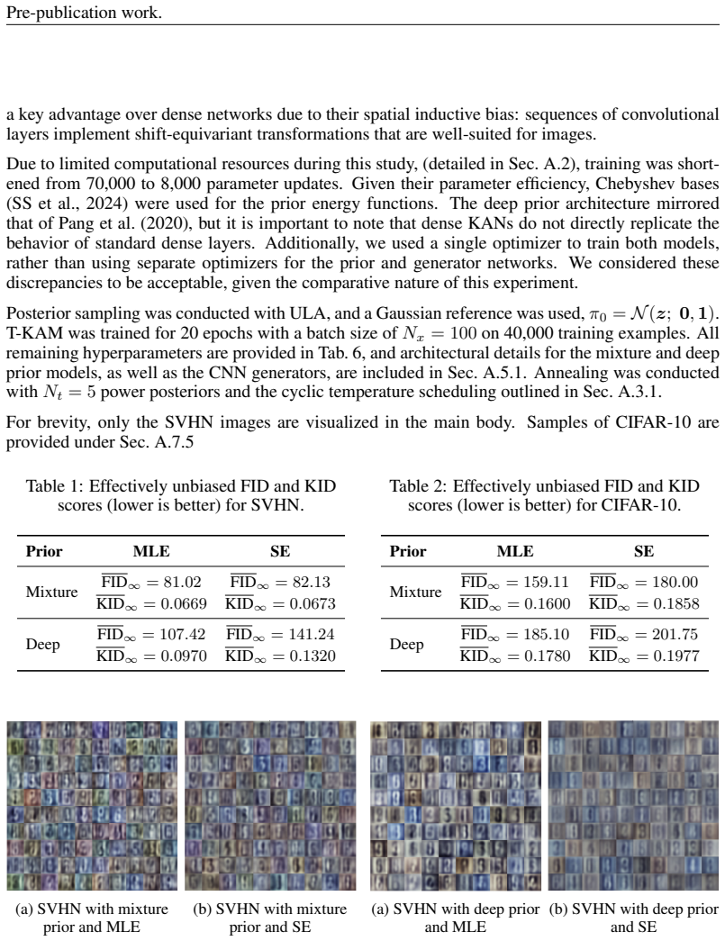
The Kolmogorov-Arnold Energy Model imposes a univariate latent structure on the energy function by adapting the Kolmogorov-Arnold Representation Theorem. This enables exact inference via the inverse transform method and makes importance sampling a tractable way to perform unbiased posterior inference. For cases of poor mixing, a population-based annealed strategy is introduced. On SVHN and CIFAR10, KAEM achieves the best Fréchet Inception Distance among compared latent-prior models, with sampling performed in a single forward pass.
What carries the argument
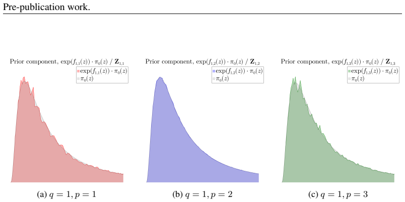
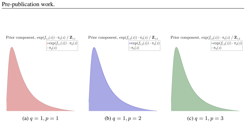
The Kolmogorov-Arnold adapted energy function that decomposes into univariate functions, carrying the argument by creating an interpretable product prior over low-dimensional latents.
If this is right
- Sampling reduces to a single forward pass through the model.
- The prior can be inspected as independent one-dimensional densities.
- Posterior inference is possible via unbiased importance sampling without MCMC.
- Performance on image generation benchmarks exceeds that of standard VAEs and neural latent EBMs.
Where Pith is reading between the lines
- This univariate decomposition might generalize to other representation theorems for even simpler structures.
- In applications requiring uncertainty quantification, the explicit 1D densities could aid in understanding model confidence.
- Future work could test whether the annealed population strategy scales to higher-dimensional or more complex data distributions.
Load-bearing premise
The assumption that a low-dimensional univariate latent structure retains sufficient modeling capacity for the complexity of natural image distributions.
What would settle it
A direct comparison on a more challenging dataset such as ImageNet where KAEM's FID scores fall significantly below those of diffusion models even with the proposed inference techniques.
Figures


read the original abstract
Generative models typically rely on either simple latent priors (e.g., Variational Autoencoders, VAEs), which are efficient but limited, or highly expressive iterative samplers (e.g., Diffusion and Energy-based Models), which are costly and opaque. We introduce the Kolmogorov-Arnold Energy Model (KAEM) to bridge this trade-off and provide new opportunities for latent-space interpretability. Based on a novel adaptation of the Kolmogorov-Arnold Representation Theorem, KAEM imposes a univariate latent structure on the prior, enabling exact inference via the inverse transform method. With a low-dimensional latent space and appropriate inductive biases, importance sampling becomes a tractable, unbiased, and efficient posterior inference method. For settings where this fails, we propose a population-based strategy that decomposes the posterior into a sequence of annealed distributions, a new remedy for poor mixing in Energy-based Models. We compare KAEM against VAEs and the neural latent EBM architecture. KAEM attains the best Fr\'echet Inception Distance among latent-prior models on SVHN and CIFAR10, while sampling in a single forward pass and exposing an interpretable prior built from 1D densities.
Editorial analysis
A structured set of objections, weighed in public.
Referee Report
Summary. The manuscript introduces Kolmogorov-Arnold Energy Models (KAEM), a generative modeling approach that adapts the Kolmogorov-Arnold Representation Theorem to impose a univariate latent structure on the energy-based prior. This structure is claimed to enable exact inference via the inverse transform method from 1D densities, tractable importance sampling for posterior inference, and a population-based annealing strategy for cases of poor mixing. KAEM is positioned as bridging simple latent priors (e.g., VAEs) and expressive iterative samplers (e.g., diffusion or EBMs), with empirical claims of achieving the best Fréchet Inception Distance among latent-prior models on SVHN and CIFAR10 while supporting single forward-pass sampling and interpretability through the 1D density components.
Significance. If the KART adaptation and empirical results hold, the work offers a meaningful contribution by combining single-pass sampling efficiency, unbiased importance sampling, and latent-space interpretability in a manner not standard in current latent-variable generative models. The explicit construction from univariate functions and the annealing remedy for mixing issues represent concrete technical advances that could influence future designs of interpretable energy-based models.
major comments (2)
- [Experimental Evaluation] Experimental section: the central claim that KAEM attains the best FID among latent-prior models on SVHN and CIFAR10 is presented without error bars, standard deviations across multiple runs, ablation studies isolating the KART prior components, or details on training stability and hyperparameter sensitivity. This absence directly weakens the ability to attribute performance gains to the proposed univariate structure rather than implementation artifacts or post-hoc tuning.
- [Model Definition / Prior Construction] Prior construction (around the KART adaptation section): the claim that the finite-sum univariate outer and inner functions preserve sufficient expressivity for modeling statistical dependencies in CIFAR10-level data rests on an untested assumption. If cross-dimensional correlations are primarily captured by the decoder rather than the prior, the reported FID improvements and the interpretability selling point would not be attributable to the univariate latent structure, threatening both the efficiency and the novelty claims.
minor comments (2)
- [Abstract] The abstract states comparisons against VAEs and neural latent EBMs but does not name the precise baseline architectures, latent dimensions, or training protocols used for those comparisons.
- [Model Definition] Notation for the univariate functions and the energy formulation could be clarified with an explicit equation showing how the Kolmogorov-Arnold sum is turned into a density or energy function.
Simulated Author's Rebuttal
We thank the referee for their constructive comments on our manuscript. We address the major comments point by point below and outline the revisions we plan to make.
read point-by-point responses
-
Referee: Experimental section: the central claim that KAEM attains the best FID among latent-prior models on SVHN and CIFAR10 is presented without error bars, standard deviations across multiple runs, ablation studies isolating the KART prior components, or details on training stability and hyperparameter sensitivity. This absence directly weakens the ability to attribute performance gains to the proposed univariate structure rather than implementation artifacts or post-hoc tuning.
Authors: We agree with the referee that the experimental evaluation would benefit from additional statistical rigor. In the revised manuscript, we will include error bars and report standard deviations from at least three independent runs for the FID scores on both SVHN and CIFAR10. We will also conduct and report ablation studies that remove or modify the KART components to isolate their contribution to performance. Furthermore, we will provide more details on training procedures, stability, and hyperparameter sensitivity in the appendix. These changes will help attribute the gains more clearly to the proposed method. revision: yes
-
Referee: Prior construction (around the KART adaptation section): the claim that the finite-sum univariate outer and inner functions preserve sufficient expressivity for modeling statistical dependencies in CIFAR10-level data rests on an untested assumption. If cross-dimensional correlations are primarily captured by the decoder rather than the prior, the reported FID improvements and the interpretability selling point would not be attributable to the univariate latent structure, threatening both the efficiency and the novelty claims.
Authors: We appreciate this insightful observation regarding the source of expressivity. The adaptation of the Kolmogorov-Arnold Representation Theorem is intended to provide a structured prior that can capture dependencies through univariate functions, as guaranteed by the theorem in the infinite case and approximated in the finite sum. Our empirical results on CIFAR10, which has complex correlations, support that the overall model benefits from this structure. However, to directly test the assumption, we will add in the revision a discussion and possibly additional experiments analyzing the learned univariate functions and their impact on latent correlations, such as by comparing correlation matrices or visualizing the 1D densities. We believe the interpretability of the 1D priors remains a valid contribution even if some correlations are handled by the decoder. revision: partial
Circularity Check
No circularity: derivation rests on external KART theorem
full rationale
The paper adapts the Kolmogorov-Arnold Representation Theorem (an external 1950s result) to impose a univariate latent structure on the energy-based prior, enabling inverse-transform sampling and tractable importance sampling. This construction is presented as a novel application rather than a self-referential definition or fitted parameter renamed as prediction. No self-citation chains, uniqueness theorems from the same authors, or ansatz smuggling appear in the abstract or described claims. Empirical FID results on SVHN/CIFAR10 are reported as comparisons against VAEs and neural latent EBMs without evidence that evaluation metrics are reused as inputs. The derivation chain remains self-contained against external mathematical benchmarks and does not reduce to its own fitted values by construction.
Axiom & Free-Parameter Ledger
axioms (1)
- domain assumption Kolmogorov-Arnold Representation Theorem can be adapted to define a valid probability density over a low-dimensional latent space for generative modeling
Lean theorems connected to this paper
-
IndisputableMonolith/Cost/FunctionalEquation.leanwashburn_uniqueness_aczel unclear?
unclearRelation between the paper passage and the cited Recognition theorem.
We interpret up ∼ U(up;0,1) ... ψq,p(up)=F⁻¹(πq,p)(up) ... πq,p(z)=exp(fq,p(z))/Zq,p ⋅ π0(z)
-
IndisputableMonolith/Foundation/RealityFromDistinction.leanreality_from_one_distinction unclear?
unclearRelation between the paper passage and the cited Recognition theorem.
novel adaptation of the Kolmogorov–Arnold Representation Theorem ... univariate energy-based prior
What do these tags mean?
- matches
- The paper's claim is directly supported by a theorem in the formal canon.
- supports
- The theorem supports part of the paper's argument, but the paper may add assumptions or extra steps.
- extends
- The paper goes beyond the formal theorem; the theorem is a base layer rather than the whole result.
- uses
- The paper appears to rely on the theorem as machinery.
- contradicts
- The paper's claim conflicts with a theorem or certificate in the canon.
- unclear
- Pith found a possible connection, but the passage is too broad, indirect, or ambiguous to say the theorem truly supports the claim.
Reference graph
Works this paper leans on
-
[1]
Auto-Encoding Variational Bayes
doi: 10.1143/jpsj.65.1604. URL http://dx.doi.org/10.1143/JPSJ.65.1604. JuliaCI. Benchmarktools.jl, 2024. URL https://juliaci.github.io/ BenchmarkTools.jl/stable/. Accessed on August 20, 2024. George Em Karniadakis, Ioannis G. Kevrekidis, Lu Lu, Paris Perdikaris, Sifan Wang, and Liu Yang. Physics-informed machine learning. Nature Reviews Physics , 3(6):422...
work page internal anchor Pith review Pith/arXiv arXiv doi:10.1143/jpsj.65.1604 2024
-
[2]
doi: 10.1090/S0025-5718-97-00861-2. Yann LeCun, Yoshua Bengio, and Geoffrey Hinton. Deep learning. Nature, 521(7553):436–444, May 28 2015. ISSN 1476-4687. doi: 10.1038/nature14539. Ziyao Li. Kolmogorov-arnold networks are radial basis function networks, 2024. URL https: //arxiv.org/abs/2405.06721. Zongyi Li, Nikola Kovachki, Kamyar Azizzadenesheli, Burige...
-
[3]
Integer replication: The sample, s, is replicated rs times, where: rs = j Ns · wnorm(z(s)) k (68)
-
[4]
Residual weights: The total number of replicated samples after the previous stage will bePNs s=1 rs. Therefore, Ns −PNs s=1 rs remain, which must be resampled using the residuals: wresidual(z(s)) = wnorm(z(s)) · (Ns − rs) wnorm, residual(z(s)) = wresidual(z(s))PNs s=1 wresidual(z(s)) (69) If a sample has been replicated at the previous stage, then its cor...
-
[5]
(70) where k∗ represents the index of the sample to keep
Resample: The remaining samples are drawn with multinomial resampling, based on the cumulative distribution function of the residuals: k∗ = min ( j | jX s=1 wnorm, residual(z(s)) ≥ ui ) where ui ∼ U ([0, 1]). (70) where k∗ represents the index of the sample to keep. A.6.3 M ETROPOLIS -ADJUSTED LANGEVIN ALGORITHM (MALA) The Metropolis-Adjusted Langevin Alg...
work page 1998
-
[6]
Langevin diffusion: A new state z′ (i, t k) is proposed for a local chain, operating with a specific tk, using a transition kernel inspired by (overdamped) Langevin dynamics (Roberts 33 Pre-publication work. & Stramer, 2002; Brooks et al., 2011): Target: log γ z′ (i, t k) ∝ log P (x(b) | z, Φ)tk + log P (z | f) Proposal: z′ (i, t k) | z(i, t k) ∼ q z′ (i,...
work page 2002
-
[7]
MH criterion: Once Nunadjusted iterations have elapsed, Metropolis-Hastings adjustments, (MH) (Metropolis & Ulam, 1949), are introduced. The criterion for the local proposal is: rlocal = γ z′ (i, t k) q z(i, t k) | z′ (i, t k) γ z(i, t k) q z′ (i, t k) | z(i, t k) , (73)
work page 1949
-
[9]
Global Swaps: Global swaps are proposed and accepted subject to the criterion outlined in Eq. 34 Convergence Under mild regularity conditions, the local Markov chain {z(i, t k)} generated by MALA converges in distribution to P (z | x(b), f , Φ, tk) as Nlocal → ∞ . The proposal mechanism in Eq. 72 ensures that the chain mixes efficiently, particularly in h...
work page 2024
-
[10]
Acceptance thresholds: Two bounding acceptance thresholds are sampled uniformly: a, b ∼ U (a, b) ;0, 1 , (a, b) ∈ [0, 1]2, b > a (75) 34 Pre-publication work
-
[11]
Here, Beta 01 [a, b; c, d] denotes a zero-one-inflated Beta distribution
Mass matrix: Random pre-conditioning matrices are initialized per latent dimension: ε(i, t k) ∼ Beta 01 1, 1; 1 2 , 2 3 , M1/2 (i, t k , q ) p,p = ε(i, t k) · Σ−1/2 (i, t k, q ) p,p + (1 − ε(i, t k)), (76) where Σ(i, t k, q ) p,p = V ARs h ¯z(i, t k, s) q,p i . Here, Beta 01 [a, b; c, d] denotes a zero-one-inflated Beta distribution. The parameters a, b >...
-
[12]
Leapfrog proposal: The following transition is proposed for a local chain, tk, with an adaptive step size, η(i,tk): p(i, t k) ∼ N p; 0, M (i, t k) p′ (i, t k) 1/2 = p(i, t k) + η(i,tk) 2 ∇z log γ z′ (i, t k) z′ (i, t k) = z(i, t k) + η(i,tk) M −1p′ 1/2 (i, t k) ˆp(i, t k) = p′ (i, t k) 1/2 + η(i,tk) 2 ∇z log γ z′ (i, t k) p′ (i, t k) = −ˆp(i, t k), (77)
-
[13]
MH criterion: Once Nunadjusted iterations have elapsed, Metropolis-Hastings (MH) adjust- ments are introduced. The MH acceptance criterion for the local proposal is: rlocal = γ z′ (i, t k) N p′ (i, t k); 0, M (i, t k) γ z(i, t k) N p(i, t k); 0, M (i, t k) , (78)
-
[14]
Step size adaptation: Starting with an initial estimate, η(i,tk) init , set as the average accepted step size from the previous training iteration, (used as a simple alternative to the round- based tuning algorithm proposed by Biron-Lattes et al. (2024)), the step size is adjusted as follows: • If a < r local < b, then η(i,tk) = η(i,tk) init • If rlocal ≤...
work page 2024
-
[15]
77 is verified before proceeding with MH acceptance
Reversibility check: If the step size was modified, the reversibility of the update in Eq. 77 is verified before proceeding with MH acceptance. If η(i,tk) init cannot be recovered from the reversed step-size adjustment process with the proposed state, z′ (i, t k), p ′ (i, t k), η(i,tk) , the proposal is rejected regardless of the outcome of the MH adjustment
-
[16]
Acceptance: The proposal is accepted with probability min(1, rlocal). If accepted, z(i+1, t k) = z′ (i, t k); otherwise, the current state is retained: z(i+1, t k) = z(i, t k)
-
[17]
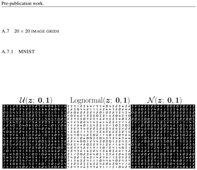
Global Swaps: Global swaps are proposed and accepted subject to Eq. 34 35 Pre-publication work. A.7 20 × 20 IMAGE GRIDS A.7.1 MNIST Figure 13: Generated MNIST, (Deng, 2012), after 2,000 parameter updates using MLE / IS adhering to KART’s structure. Uniform, lognormal, and Gaussian priors are contrasted using Radial Basis Functions, (Li, 2024). Lognormal i...
work page 2012
discussion (0)
Sign in with ORCID, Apple, or X to comment. Anyone can read and Pith papers without signing in.