HiPreNets: High-Precision Neural Networks through Progressive Training
Pith reviewed 2026-05-19 09:36 UTC · model grok-4.3
The pith
HiPreNets progressively trains refinement networks on normalized residuals to reduce both average and worst-case errors toward machine precision.
A machine-rendered reading of the paper's core claim, the machinery that carries it, and where it could break.
Core claim
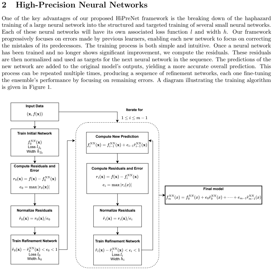
Sequential residual refinement reduces both RMSE and L^∞ norm error more effectively than conventional training by training each new network on the normalized residuals of the current ensemble and by concentrating updates on high-error regions through complementary techniques including loss design, adaptive data sampling, localized patching, and boundary-aware training.
What carries the argument
Progressive residual refinement ensemble, in which each stage trains a new network on the normalized difference between the present ensemble output and the target values.
If this is right
- Higher final accuracy is obtained on nonlinear regression tasks without a proportional increase in total model capacity.
- Lower maximum errors make the models more suitable for safety-critical engineering applications.
- Fast, high-fidelity surrogate models become feasible for high-dimensional dynamical systems such as power-grid ODEs.
- Consistent gains appear across both low-dimensional physics benchmarks and higher-dimensional simulation problems.
Where Pith is reading between the lines
- The method might be combined with other base architectures to further improve results on the same benchmarks.
- Testing on problems with dimensions substantially above 20 could expose whether error reduction remains stable or saturates.
- The explicit focus on L^∞ reduction could be paired with physics-informed loss terms for additional accuracy gains in scientific modeling.
- The progressive structure suggests a natural way to allocate compute adaptively across different regions of high-dimensional input spaces.
Load-bearing premise
Successive refinement networks trained on normalized residuals will keep lowering both average and maximum errors over the whole input domain without instability, overfitting, or prohibitive growth in training cost as dimension or complexity rises.
What would settle it
A clear test case in which additional refinement stages cease to decrease, or begin to increase, the L^∞ error on any region of the input domain for a Feynman benchmark problem.
Figures


read the original abstract
Deep neural networks are powerful tools for solving nonlinear problems in science and engineering, but training highly accurate models becomes challenging as problem complexity increases. Non-convex optimization and sensitivity to hyperparameters make consistent performance improvement difficult, and traditional approaches prioritize minimizing mean squared error while overlooking the $L^{\infty}$ norm error that is critical in safety-sensitive applications. To address these challenges, we present HiPreNets, a progressive framework for training high-precision neural networks through sequential residual refinements. Starting from an initial network, each stage trains a refinement network on the normalized residuals of the ensemble so far, systematically reducing both average and worst-case error. A key theme throughout the framework is concentrating training effort on high-error regions of the input domain, which we pursue through complementary techniques including loss function design, adaptive data sampling, localized patching, and boundary-aware training. We validate the framework on benchmark regression problems from the Feynman dataset, where it consistently outperforms standard fully connected networks and reported Kolmogorov-Arnold Networks results, with accuracy approaching machine precision depending on select problems. We further apply the framework to learning the flow map of a 20-dimensional power system ODE, which appears to be the highest dimensional problem studied using this class of multistage methods, achieving substantial reductions in both RMSE and $L^{\infty}$ norm error while enabling a surrogate that predicts system state $238\times$ faster than direct numerical simulation.
Editorial analysis
A structured set of objections, weighed in public.
Referee Report
Summary. The paper introduces HiPreNets, a progressive framework for high-precision neural networks. It begins with an initial network and trains successive refinement networks on the normalized residuals of the current ensemble, employing adaptive sampling, localized patching, and boundary-aware training to concentrate effort on high-error regions. Validation is reported on Feynman dataset regression tasks, where the method outperforms standard fully connected networks and published Kolmogorov-Arnold Network results with accuracy approaching machine precision on select problems, and on learning the flow map of a 20-dimensional power-system ODE, where it achieves substantial RMSE and L^∞ error reductions while delivering a surrogate 238 times faster than direct numerical simulation.
Significance. If the central performance claims hold under scrutiny, the work would be significant for scientific machine learning, offering a practical route to high-precision surrogates in safety-critical and high-dimensional settings where L^∞ error control matters. The emphasis on progressive residual refinement with focused sampling addresses a recognized limitation of standard MSE-trained networks. The 20D power-system example is presented as the highest-dimensional multistage case studied, which, if supported by detailed diagnostics, would strengthen the case for scalability.
major comments (3)
- [Abstract and §4] Abstract and §4: The headline claims of approaching machine precision on Feynman subsets and substantial L^∞ reductions on the 20D problem are stated without accompanying quantitative tables, error bars, ablation results, or explicit numerical values for RMSE and L^∞ before/after each stage. This absence makes it impossible to verify the magnitude and consistency of the reported improvements.
- [§3] §3 (Framework description): The procedure treats the number of refinement stages and the residual normalization scale as free parameters. The manuscript does not specify selection criteria or demonstrate robustness to these choices; without such analysis the claim that refinements 'systematically' reduce both average and worst-case error rests on an incompletely characterized procedure.
- [§4.2] §4.2 (20D power-system experiment): The reported 238× speedup and error reductions are presented as a single-point outcome. No per-stage error curves, ablation removing adaptive sampling or boundary-aware terms, or analysis of behavior once residuals approach floating-point noise are supplied. This directly bears on whether successive refinements continue to drive L^∞ error downward without plateau or instability in 20D.
minor comments (2)
- [§3] Notation: The distinction between the ensemble prediction and the residual target at each stage should be made explicit with consistent symbols across equations and text.
- [Figure 1] Figures: The schematic of the progressive training loop would benefit from explicit annotation of the normalization step and the adaptive sampling region.
Simulated Author's Rebuttal
We thank the referee for the constructive and detailed comments. We address each major point below and indicate the revisions planned for the next version of the manuscript.
read point-by-point responses
-
Referee: [Abstract and §4] Abstract and §4: The headline claims of approaching machine precision on Feynman subsets and substantial L^∞ reductions on the 20D problem are stated without accompanying quantitative tables, error bars, ablation results, or explicit numerical values for RMSE and L^∞ before/after each stage. This absence makes it impossible to verify the magnitude and consistency of the reported improvements.
Authors: We agree that the current manuscript would benefit from more explicit quantitative support. In the revised version we will add tables in §4 that report RMSE and L^∞ values at each refinement stage for the Feynman benchmarks, together with error bars obtained from multiple independent runs. For the 20D power-system example we will likewise tabulate the per-stage error reductions and the final speedup factor. revision: yes
-
Referee: [§3] §3 (Framework description): The procedure treats the number of refinement stages and the residual normalization scale as free parameters. The manuscript does not specify selection criteria or demonstrate robustness to these choices; without such analysis the claim that refinements 'systematically' reduce both average and worst-case error rests on an incompletely characterized procedure.
Authors: The referee is correct that these quantities are hyperparameters. We will expand §3 to state explicit stopping criteria (e.g., continue while the validation residual exceeds a threshold near machine precision or until error plateaus) and will add a short robustness study that varies the number of stages and normalization scale on representative problems, confirming that the observed error reductions remain consistent. revision: yes
-
Referee: [§4.2] §4.2 (20D power-system experiment): The reported 238× speedup and error reductions are presented as a single-point outcome. No per-stage error curves, ablation removing adaptive sampling or boundary-aware terms, or analysis of behavior once residuals approach floating-point noise are supplied. This directly bears on whether successive refinements continue to drive L^∞ error downward without plateau or instability in 20D.
Authors: We acknowledge the value of these additional diagnostics. The revised §4.2 will include per-stage RMSE and L^∞ curves, ablations that isolate the contribution of adaptive sampling and boundary-aware training, and a brief analysis of error behavior as residuals approach floating-point limits, showing that further stages do not introduce instability. revision: yes
Circularity Check
No circularity: HiPreNets is a standard multi-stage residual refinement procedure relying on conventional NN optimization.
full rationale
The paper presents HiPreNets as a sequential training process that starts with an initial network and adds refinement networks trained on normalized residuals of the current ensemble, using adaptive sampling and localized patching to target high-error regions. This is an empirical engineering framework built on standard neural-network training loops and loss design rather than any first-principles derivation or mathematical claim that reduces to its own inputs by construction. No equations define a target quantity in terms of itself, no fitted parameters are relabeled as predictions, and no load-bearing uniqueness theorems or ansatzes are imported via self-citation. Performance results on Feynman benchmarks and the 20D power-system ODE are presented as empirical outcomes, not as tautological consequences of the method's own definitions. The derivation chain is therefore self-contained against external benchmarks.
Axiom & Free-Parameter Ledger
free parameters (2)
- number of refinement stages
- residual normalization scale
axioms (2)
- standard math Neural networks are universal approximators for continuous functions on compact sets.
- domain assumption Normalized residuals from an ensemble can be learned by an additional network without destabilizing prior stages.
Reference graph
Works this paper leans on
-
[1]
S. Abrecht, A. Hirsch, S. Raafatnia, and M. Woehrle. Deep learning safety concerns in automated driving perception. IEEE Transactions on Intelligent Vehicles , 2024
work page 2024
-
[2]
Concrete Problems in AI Safety
D. Amodei, C. Olah, J. Steinhardt, P. Christiano, J. Schulman, and D. Man´ e. Concrete problems in ai safety. arXiv preprint arXiv:1606.06565 , 2016
work page internal anchor Pith review Pith/arXiv arXiv 2016
- [3]
-
[4]
S. Badirli, X. Liu, Z. Xing, A. Bhowmik, K. Doan, and S. S. Keerthi. Gradient boosting neural networks: Grownet. arXiv preprint arXiv:2002.07971 , 2020
-
[5]
Y. Bengio. Gradient-based optimization of hyperparameters. Neural computation, 12(8):1889–1900, 2000
work page 1900
-
[6]
L. Breiman, J. H. Friedman, R. A. Olshen, and C. J. Stone. Classification and regression trees. 1984
work page 1984
-
[7]
T. Chen and C. Guestrin. Xgboost: A scalable tree boosting system. In Proceedings of the 22nd acm sigkdd international conference on knowledge discovery and data mining , pages 785–794, 2016
work page 2016
-
[8]
A. Choromanska, M. Henaff, M. Mathieu, G. B. Arous, and Y. LeCun. The loss surfaces of multilayer networks. In Artificial intelligence and statistics , pages 192–204. PMLR, 2015
work page 2015
-
[9]
V. G. Costa and C. E. Pedreira. Recent advances in decision trees: An updated survey. Artificial Intelligence Review, 56(5):4765–4800, 2023
work page 2023
-
[10]
Y. N. Dauphin, R. Pascanu, C. Gulcehre, K. Cho, S. Ganguli, and Y. Bengio. Identifying and attacking the saddle point problem in high-dimensional non-convex optimization. Advances in neural information processing systems, 27, 2014. 24
work page 2014
-
[11]
C. Dong, L. Zheng, and W. Chen. Kolmogorov-arnold networks (kan) for time series classification and robust analysis. In Advanced Data Mining and Applications: 20th International Conference, ADMA 2024, Sydney, NSW, Australia, December 3–5, 2024, Proceedings, Part IV , page 342–355, Berlin, Hei- delberg, 2024. Springer-Verlag
work page 2024
-
[12]
J. H. Friedman. Greedy function approximation: a gradient boosting machine. Annals of statistics , pages 1189–1232, 2001
work page 2001
-
[13]
Q. Gong, W. Kang, and F. Fahroo. Approximation of compositional functions with relu neural networks. Systems & Control Letters , 175:105508, 2023
work page 2023
-
[14]
I. Goodfellow, J. Shlens, and C. Szegedy. Explaining and harnessing adversarial examples. In Interna- tional Conference on Learning Representations, 2015
work page 2015
- [15]
-
[16]
W. Kang and Q. Gong. Feedforward neural networks and compositional functions with applications to dynamical systems. SIAM Journal on Control and Optimization , 60(2):786–813, 2022
work page 2022
-
[17]
A. N. Kolmogorov. On the representation of continuous functions of several variables by superpositions of continuous functions of one variable and addition. Doklady Akademii Nauk SSSR , 114:953–956, 1957
work page 1957
-
[18]
A. Krizhevsky, I. Sutskever, and G. E. Hinton. Imagenet classification with deep convolutional neural networks. Advances in neural information processing systems , 25, 2012
work page 2012
-
[19]
Z. Liu, Y. Wang, S. Vaidya, F. Ruehle, J. Halverson, M. Soljacic, T. Y. Hou, and M. Tegmark. KAN: Kolmogorov–arnold networks. In The Thirteenth International Conference on Learning Representations, 2025
work page 2025
-
[20]
E. J. Michaud, Z. Liu, and M. Tegmark. Precision machine learning. Entropy, 25(1):175, 2023
work page 2023
-
[21]
J. Nocedal and S. Wright. Numerical Optimization. Springer Science & Business Media, 2nd edition, 2006
work page 2006
-
[22]
J. R. Quinlan. Induction of decision trees. Machine learning, 1:81–106, 1986
work page 1986
-
[23]
J. R. Quinlan. C4.5: Programs for Machine Learning. Morgan Kaufmann Publishers Inc., San Francisco, CA, USA, 1993
work page 1993
-
[24]
A. Radford, K. Narasimhan, T. Salimans, I. Sutskever, et al. Improving language understanding by generative pre-training. 2018
work page 2018
-
[25]
N. Rahaman, A. Baratin, D. Arpit, F. Draxler, M. Lin, F. Hamprecht, Y. Bengio, and A. Courville. On the spectral bias of neural networks. In International conference on machine learning, pages 5301–5310. PMLR, 2019
work page 2019
-
[26]
F. Rosenblatt. The perceptron: A perceiving and recognizing automaton. Report, Project PARA, Cornell Aeronautical Laboratory, Jan. 1957
work page 1957
-
[27]
D. E. Rumelhart, G. E. Hinton, and R. J. Williams. Learning representations by back-propagating errors. nature, 323(6088):533–536, 1986
work page 1986
- [28]
- [29]
-
[30]
S.-M. Udrescu and M. Tegmark. Ai feynman: A physics-inspired method for symbolic regression. Science Advances, 6(16):eaay2631, 2020. 25
work page 2020
-
[31]
A. Vaswani, N. Shazeer, N. Parmar, J. Uszkoreit, L. Jones, A. N. Gomez, L. u. Kaiser, and I. Polo- sukhin. Attention is all you need. In I. Guyon, U. V. Luxburg, S. Bengio, H. Wallach, R. Fergus, S. Vishwanathan, and R. Garnett, editors, Advances in Neural Information Processing Systems , vol- ume 30. Curran Associates, Inc., 2017
work page 2017
-
[32]
P. Virtanen, R. Gommers, T. E. Oliphant, M. Haberland, T. Reddy, D. Cournapeau, E. Burovski, P. Peterson, W. Weckesser, J. Bright, S. J. van der Walt, M. Brett, J. Wilson, K. J. Millman, N. Mayorov, A. R. J. Nelson, E. Jones, R. Kern, E. Larson, C. J. Carey,˙I. Polat, Y. Feng, E. W. Moore, J. VanderPlas, D. Laxalde, J. Perktold, R. Cimrman, I. Henriksen, ...
work page 2020
-
[33]
Y. Wang and C.-Y. Lai. Multi-stage neural networks: Function approximator of machine precision. Journal of Computational Physics , 504:112865, 2024
work page 2024
-
[34]
S. Xie, R. Girshick, P. Doll´ ar, Z. Tu, and K. He. Aggregated residual transformations for deep neural networks. In Proceedings of the IEEE conference on computer vision and pattern recognition , pages 1492–1500, 2017
work page 2017
- [35]
discussion (0)
Sign in with ORCID, Apple, or X to comment. Anyone can read and Pith papers without signing in.