REVIEW 4 major objections 5 minor 48 references
Acoustic Waveform Inversion with Image-to-Image Schr\"odinger Bridges
T0 review · 4 major / 5 minor · reviewed 2026-08-15 · deepseek-v4-flash
Pith's one-line read A conditional Schrödinger bridge turns a smoothed velocity model into a posterior sample over ground truth using only a few network evaluations.
desk verdict A credible application paper that borrows its theory from cDSB/I2SB and delivers a useful FWI demo, but the headline posterior guarantee only holds under a distortion prior the authors admit is unrealistic. read the letter →
The pith
A machine-rendered reading of the paper's core claim, the machinery that carries it, and where it could break.
The reading
What carries the argument
The central object is the conditional Image-to-Image Schrödinger Bridge (cI2SB): a Schrödinger bridge interpolating between the distribution of ground-truth velocity models and the distribution of smoothed velocity models, with the observed seismic data serving as a conditioning variable that does not evolve along the bridge (dy = 0). The load-bearing identity is the analytic posterior q(xt|x0,x1) of the I2SB formulation, which lets the model sample intermediate velocity states directly during training and gives the DDPM-style recursion used at inference. The training procedure (Alg. 2) learns conditional and unconditional drifts in a single network, alternating between prediction with and without the data channel, and the sampling procedure (Alg. 3) blends the two predictions with a guidance scale η. This machinery converts the previously heuristic 'how to include the initial velocity model' into a boundary condition of a stochastic optimal transport problem.
What would settle it
Run the released cI2SB model starting from a smooth velocity model produced by a different mechanism than pdist — for example, migration or traveltime tomography, or a Gaussian blur with kernel size 16–24 or 0–8 — and compare MAE/MSE/SSIM with the in-distribution results in Tables 2–3; a drop to the levels of Table 6's out-of-distribution rows would falsify the claim that the inference is a general posterior sampler rather than a memorization of the training distortion.
Extended reading notes
Core claim
The central claim is that the cI2SB framework, derived from the amortized conditional Schrödinger bridge problem, provides an acoustic FWI scheme whose inference starts from a smoothed velocity model and terminates at a sample from the posterior over ground-truth velocity models conditioned on observed seismic data, and that on OpenFWI this scheme outperforms a reimplemented conditional diffusion model while reaching sample fidelity superior to a supervised approach with only a few neural function evaluations. The bridge is constructed by fixing the forward reference measure to the acoustic velocity field while the seismic data channel stays constant, and by taking the endpoint prior to be the parametric distortion pdist(c1|c0) applied to ground truth. Because the bridge posterior q(ct|c0,c1) is analytic, training reduces to denoising score matching with paired (c0, c1, dobs) triples, and inference runs the DDPM recursion backward from csmooth. The authors report that the guidance scale η controls the diversity of reconstructed velocity fields, and that objective reweighting (wcond) is necessary to keep the network attending to the seismic data.
Load-bearing premise
The load-bearing premise is that a real-world smoothed velocity model is a sample from the Gaussian-blur-plus-noise distortion family used in training; the paper states this construction has no basis in real-world data, and its Table 6 shows performance degrades when the smoothing kernel leaves the training range.
Editorial extensions
If this is right
- Diffusion-based acoustic inversion can start from an arbitrary smoothed velocity model and still be guaranteed, in the continuous-time limit, to produce a posterior sample over true velocity models given the observed data.
- The cost of high perceptual fidelity drops from hundreds of network evaluations (typical for Gaussian-prior diffusion) to roughly 5–50, making the method practical for large 2D surveys.
- The guidance scale η gives practitioners a single hyperparameter to trade sample diversity against fidelity, with η = 1 collapsing the output to a near-deterministic reconstruction.
- Because the distortion operator is explicit, the same framework can be retargeted to other 'smooth start' priors — migration images, tomography models — by retraining with a matching pdist.
- At matched NFEs, the bridge model consistently beats the conditional diffusion baseline on all tested OpenFWI dataset families by a statistically significant margin.
Reading between the lines
- We infer that the same conditional-bridge construction should transfer to other seismic inverse problems (elastic FWI, migration-image conditioning) wherever a paired smooth-to-true training set exists, since the method only needs pjoin and pdist.
- The paper's Table 6 suggests a practical calibration recipe: before field deployment, measure the actual distortion between available smooth models and true velocity using wells, and retrain the bridge with that empirical pdist; otherwise the endpoint guarantee does not apply.
- The authors' observation that the network ignores the data channel unless wcond is large hints at a general pitfall: with informative priors, joint conditional/unconditional training is biased toward the unconditional solution, and explicit loss reweighting may be needed in any bridge-based posterior sampler.
Signed reviews
Editorial analysis
A structured set of objections, weighed in public.
Referee Report
Summary. The paper proposes cI2SB, a conditional Image-to-Image Schrödinger Bridge for acoustic full waveform inversion. It adapts the I2SB training objective to take seismic data and a smoothed velocity model as conditional inputs, and uses a classifier-free guidance style weighting to trade off conditional and unconditional denoising. The inference starts from a smoothed velocity model and terminates at a sample from the learned posterior over velocity models conditioned on the seismic data. Experiments on OpenFWI subsets compare the method against InversionNet and a reimplemented conditional SGM, reporting improved SSIM and sample fidelity with a few NFEs. The paper also studies the effect of NFE count and guidance scale.
Significance. If the empirical claims hold, the paper provides a more principled way to incorporate initial velocity models into diffusion-based FWI than current heuristics, and the few-NFE property is practically valuable. The derivation is a straightforward application of the cDSB framework to the I2SB setting, and the authors are transparent about the synthetic nature of the distortion prior. Strengths include a reproducible code repository, a clean statement of the theoretical backbone, and a systematic NFE study. However, the central guarantee is conditional on the training distortion operator, which the authors admit has no real-world basis; this limits the significance unless addressed.
major comments (4)
- [Section 5.1.3 and Section 6.4] The distortion operator D^γ_k of Eq. (25) is explicitly described as 'not hav[ing] any basis in real-world data', and Table 6 shows that using different kernel sizes degrades performance. The theoretical guarantee that the inference process ends at a posterior sample (stated in the Abstract and Section 3) holds only when the initial smoothed model is drawn from the same parametric distortion family used in training. For real FWI initial models from migration or tomography, whose errors are structured and spatially correlated, there is no reason the bridge endpoint will be the posterior. The paper should either incorporate a physics-based data-consistency term into the loss or sampling, or explicitly reframe the main claim as conditional on the distortion model.
- [Section 5.2 and Tables 2-3] The claim that cI2SB 'outperforms' the conditional SGM 'by statistically significant margin' is not supported by the reported results. No error bars or repeated runs are provided for the deterministic baselines (InversionNet and cSGM); only the stochastic cI2SB results are averaged over 50 seeds, but their variance is not reported. Moreover, in Table 3, for FlatVelA the cSGM reports lower MAE and MSE than cI2SB OT-ODE sampling, so the statement 'in all studied cases' is factually inaccurate. Please provide confidence intervals or a proper statistical comparison, and soften the claim accordingly.
- [Tables 4 and 5] The NFE study contains numerical inconsistencies that undermine the quantitative claims. For example, in Table 4 the FlatVelB row at NFE=1 lists MAE=1.63e-2 and MSE=1.71e-2, which is impossible for normalized data; in Table 5 the FlatFaultB row at NFE=50 lists MAE=3.46e-3, an order of magnitude lower than the neighboring rows, suggesting a missing digit. Please correct these values and re-verify all numbers.
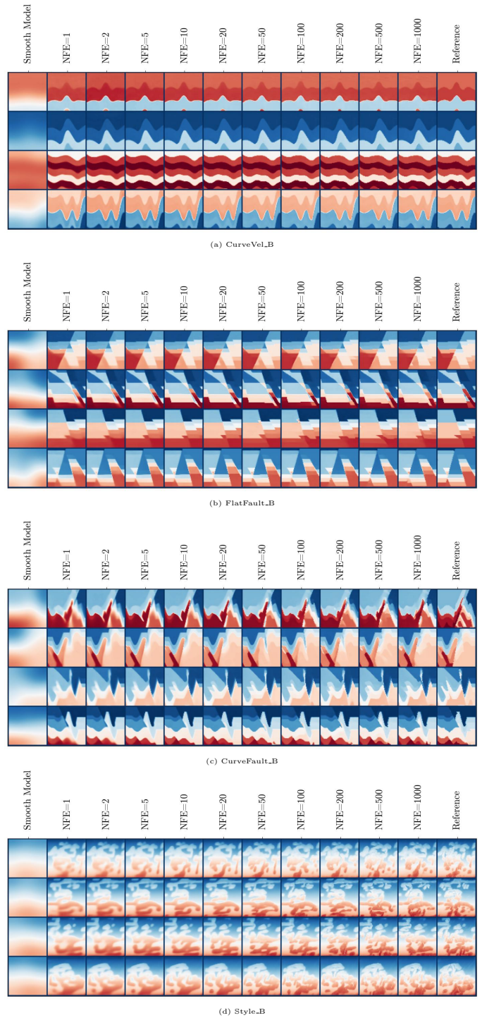
- [Section 6.2] The claim that cI2SB achieves superior perceptual quality with fewer NFEs is supported only by visual inspection of Fig. 12. To make this claim quantitative, please report a perceptual metric such as FID or LPIPS, or at least report the variance of the standard metrics over the validation set.
minor comments (5)
- [Equation (17)] The variance terms σ^2_t and σ^2_t use identical notation, which is ambiguous. Please follow the I2SB convention of σ_t^2 and σ̄_t^2.
- [Section 5.1.4] The description of the InversionNet reimplementation as passing a constant timestep value to the network is unclear; InversionNet is not a diffusion model. Please clarify the exact architecture and training procedure used.
- [Section 5.1.1 vs. Supplementary Figure 8] The text reports wcond=100, while the caption of Figure 8 refers to wcond=10. Please reconcile this inconsistency.
- [Throughout] There are numerous typos, e.g., 'existense' in Section 1 and inconsistent rendering of 'Schrödinger' as 'Schr¨ odinger'.
- [Section 5.1.5] For the stochastic cI2SB results averaged over 50 seeds, please report standard deviations or interquartile ranges in addition to the means.
Circularity Check
No significant circularity: the cI2SB derivation is grounded in external cited theory, the training loss regresses ground truth directly, and evaluation uses external OpenFWI validation splits.
full rationale
The paper does not exhibit circular derivation. The conditional Schrödinger bridge formulation (Eqs. 13-14 and 21-24) is attributed to Shi et al. [24], and the analytic bridge posterior (Eq. 17) and the delta-measure construction in Section 2.5 are attributed to Liu et al. [25]; these are external peer-reviewed results, and the reference list contains no self-citations by Stankevich/Petrov, so no self-citation chain is load-bearing. The training objective (Algorithms 1-2) directly regresses the ground-truth velocity model c0 from the noisy bridge sample and the conditioning seismogram, and the evaluation in Tables 2-3 is performed against OpenFWI validation splits that were not used to fit model parameters; no fitted parameter is renamed as a prediction. The only qualification is an explicit and acknowledged limitation: the distortion operator in Eq. 25 is a synthetic construction ('Note, however, that suggested construction is generic and does not have any basis in real-world data', Section 5.1.3), and Section 6.4 shows that out-of-distribution smoothed models degrade inversion metrics. That is a correctness and generalization risk for real FWI inputs, not a circularity, because the paper openly states the operator's synthetic nature and does not claim the theoretical endpoint guarantee transfers to arbitrary real-world smoothed models. Thus the derivation chain is self-contained with respect to its own stated assumptions.
Assumptions & free parameters
free parameters (4)
- Distortion operator hyperparameters (k, gamma) =
k in [8,16]; gamma in [0,0.2]
- Conditional loss weight wcond =
100
- Unconditional training probability puncond =
0.5
- Guidance scale eta (sampling) =
0 to 1, user-controlled
assumptions (5)
- standard math Analytic posterior q(xt|x0,x1) in Eq. (17) is Gaussian with closed-form mean and variance under f=0 and Dirac-delta data (from Liu et al. [25]).
- standard math The amortized conditional SB problem (13) is equivalent to an extended-space SB (14), giving tractable pjoin and pjprior (from Shi et al. [24]).
- domain assumption Test-time initial velocity models csmooth are generated from the same parametric family used in training: c1 = S_k(gamma z + (1-gamma) c0), with k in [8,16] and gamma in [0,0.2].
- ad hoc to paper Joint training of conditional and unconditional drifts in one network, with zero-masking (puncond=0.5) and convex guidance combination (eta), produces valid posterior sampling control.
- domain assumption Fixed acquisition geometry and constant seismogram conditioning shape (5x64x64) across training and test.
Cite this review
Pith. "Pith review of Acoustic Waveform Inversion with Image-to-Image Schr\"odinger Bridges." pith.science (2026). https://pith.science/paper/TR5VXVY7
@misc{pith2026250615346,
  author       = {Pith},
  title        = {Pith review of: Acoustic Waveform Inversion with Image-to-Image Schr\"odinger Bridges},
  year         = {2026},
  howpublished = {\url{https://pith.science/paper/TR5VXVY7}},
  note         = {Machine review of arXiv:2506.15346}
}
abstract
Recent developments in application of deep learning models to acoustic Full Waveform Inversion (FWI) are marked by the use of diffusion models as prior distributions for Bayesian-like inference procedures. The advantage of these methods is the ability to generate high-resolution samples, which are otherwise unattainable with classical inversion methods or other deep learning-based solutions. However, the iterative and stochastic nature of sampling from diffusion models along with heuristic nature of output control remain limiting factors for their applicability. For instance, an optimal way to include the approximate velocity model into diffusion-based inversion scheme remains unclear, even though it is considered an essential part of FWI pipeline. We address the issue by employing a Schr\"odinger Bridge that interpolates between the distributions of ground truth and smoothed velocity models. To facilitate the learning of nonlinear drifts that transfer samples between distributions we extend the concept of Image-to-Image Schr\"odinger Bridge ($\text{I}^2\text{SB}$) to conditional sampling, resulting in a conditional Image-to-Image Schr\"odinger Bridge (c$\text{I}^2\text{SB}$) framework. To validate our method, we assess its effectiveness in reconstructing the reference velocity model from its smoothed approximation, coupled with the observed seismic signal of fixed shape. Our experiments demonstrate that the proposed solution outperforms our reimplementation of conditional diffusion model suggested in earlier works, while requiring only a few neural function evaluations (NFEs) to achieve sample fidelity superior to that attained with supervised learning-based approach. The supplementary code implementing the algorithms described in this paper can be found in the repository https://github.com/stankevich-mipt/seismic_inversion_via_I2SB.
Figures


Figures from the paper (10 more)



Reference graph
Works this paper leans on
-
[1]
B. H. Russell, Introduction to seismic inversion methods . SEG Books, 1988
work page 1988
-
[2]
G. T. Schuster, Seismic inversion. Society of Exploration Geophysicists, 2017
work page 2017
-
[3]
J. O. Robertsson, B. Bednar, J. Blanch, C. Kostov, and D.-J. van Manen, Introduction to the supplement on seismic modeling with applications to acquisition, processing, and interpretation , 2007
work page 2007
-
[4]
Accuracy of finite-difference modeling of the acoustic wave equa- tion,
R. Alford, K. Kelly, and D. M. Boore, “Accuracy of finite-difference modeling of the acoustic wave equa- tion,” Geophysics, vol. 39, no. 6, pp. 834–842, 1974
work page 1974
-
[5]
A. Adler, M. Araya-Polo, and T. Poggio, “Deep learning for seismic inverse problems: Toward the accel- eration of geophysical analysis workflows,” IEEE Signal Processing Magazine , vol. 38, no. 2, pp. 89–119, 2021
work page 2021
-
[6]
Applications of deep neural networks in exploration seismology: A technical survey,
S. M. Mousavi, G. C. Beroza, T. Mukerji, and M. Rasht-Behesht, “Applications of deep neural networks in exploration seismology: A technical survey,” Geophysics, vol. 89, no. 1, WA95–WA115, 2024
work page 2024
-
[7]
M. Araya-Polo, J. Jennings, A. Adler, and T. Dahlke, “Deep-learning tomography,” The Leading Edge , vol. 37, no. 1, pp. 58–66, 2018. 15
work page 2018
-
[8]
Adjoint-driven deep-learning seismic full-waveform inversion,
W. Zhang, J. Gao, Z. Gao, and H. Chen, “Adjoint-driven deep-learning seismic full-waveform inversion,” IEEE Transactions on Geoscience and Remote Sensing , vol. 59, no. 10, pp. 8913–8932, 2020
work page 2020
Show all 48 references
-
[9]
Deep-learning full-waveform inversion using seismic migration images,
W. Zhang and J. Gao, “Deep-learning full-waveform inversion using seismic migration images,” IEEE Transactions on Geoscience and Remote Sensing , vol. 60, pp. 1–18, 2021
2021
-
[10]
Inversionnet: An efficient and accurate data-driven full waveform inversion,
Y. Wu and Y. Lin, “Inversionnet: An efficient and accurate data-driven full waveform inversion,” IEEE Transactions on Computational Imaging , vol. 6, pp. 419–433, 2019
2019
-
[11]
Deep-learning inversion: A next-generation seismic velocity model building method,
F. Yang and J. Ma, “Deep-learning inversion: A next-generation seismic velocity model building method,” Geophysics, vol. 84, no. 4, R583–R599, 2019
2019
-
[12]
Data-driven seismic waveform inversion: A study on the robustness and general- ization,
Z. Zhang and Y. Lin, “Data-driven seismic waveform inversion: A study on the robustness and general- ization,” IEEE Transactions on Geoscience and Remote sensing , vol. 58, no. 10, pp. 6900–6913, 2020
2020
-
[13]
Denoising diffusion probabilistic models,
J. Ho, A. Jain, and P. Abbeel, “Denoising diffusion probabilistic models,” Advances in neural information processing systems, vol. 33, pp. 6840–6851, 2020
2020
-
[14]
Diffusion models: A comprehensive survey of methods and applica- tions,
L. Yang, Z. Zhang, Y. Song, et al., “Diffusion models: A comprehensive survey of methods and applica- tions,” ACM Computing Surveys , vol. 56, no. 4, pp. 1–39, 2023
2023
-
[15]
Score-based generative modeling through stochastic differential equations,
Y. Song, J. Sohl-Dickstein, D. P. Kingma, A. Kumar, S. Ermon, and B. Poole, “Score-based generative modeling through stochastic differential equations,” arXiv preprint arXiv:2011.13456 , 2020
2011 arXiv
-
[16]
Srdiff: Single image super-resolution with diffusion probabilistic models,
H. Li, Y. Yang, M. Chang, et al., “Srdiff: Single image super-resolution with diffusion probabilistic models,” Neurocomputing, vol. 479, pp. 47–59, 2022
2022
-
[17]
Repaint: Inpainting using denoising diffusion probabilistic models,
A. Lugmayr, M. Danelljan, A. Romero, F. Yu, R. Timofte, and L. Van Gool, “Repaint: Inpainting using denoising diffusion probabilistic models,” in Proceedings of the IEEE/CVF conference on computer vision and pattern recognition, 2022, pp. 11 461–11 471
2022
-
[18]
Denoising diffusion restoration models,
B. Kawar, M. Elad, S. Ermon, and J. Song, “Denoising diffusion restoration models,” Advances in Neural Information Processing Systems, vol. 35, pp. 23 593–23 606, 2022
2022
-
[19]
Ho and T
J. Ho and T. Salimans, Classifier-free diffusion guidance, 2022. arXiv: 2207.12598 [cs.LG]
2022 arXiv
-
[20]
Rombach, A
R. Rombach, A. Blattmann, D. Lorenz, P. Esser, and B. Ommer, High-resolution image synthesis with latent diffusion models , 2022. arXiv: 2112.10752 [cs.CV]
2022 arXiv
-
[21]
F. Wang, X. Huang, and T. A. Alkhalifah, IEEE Transactions on Geoscience and Remote Sensing, vol. 61, pp. 1–11, 2023
2023
-
[22]
Controllable seismic velocity synthesis using generative dif- fusion models,
F. Wang, X. Huang, and T. Alkhalifah, “Controllable seismic velocity synthesis using generative dif- fusion models,” Journal of Geophysical Research: Machine Learning and Computation , vol. 1, no. 3, e2024JH000153, 2024
2024
-
[23]
Diffusionvel: Multi-information integrated velocity inversion using gen- erative diffusion models,
H. Zhang, Y. Li, and J. Huang, “Diffusionvel: Multi-information integrated velocity inversion using gen- erative diffusion models,” arXiv preprint arXiv:2410.21776 , 2024
2024 arXiv
-
[24]
Conditional simulation using diffusion schr¨ odinger bridges,
Y. Shi, V. De Bortoli, G. Deligiannidis, and A. Doucet, “Conditional simulation using diffusion schr¨ odinger bridges,” in Uncertainty in Artificial Intelligence , PMLR, 2022, pp. 1792–1802
2022
-
[25]
G.-H. Liu, A. Vahdat, D.-A. Huang, E. A. Theodorou, W. Nie, and A. Anandkumar, I2sb: Image-to-image schr¨ odinger bridge, 2023. arXiv: 2302.05872 [cs.CV]
2023 arXiv
-
[26]
Openfwi: Benchmark seismic datasets for machine learning-based full waveform inversion,
C. Deng, Y. Feng, S. Feng, et al., “Openfwi: Benchmark seismic datasets for machine learning-based full waveform inversion,” CoRR, vol. abs/2111.02926, 2021. arXiv: 2111.02926
2021 arXiv
-
[27]
An overview of full-waveform inversion in exploration geophysics,
“An overview of full-waveform inversion in exploration geophysics,” Geophysics, vol. 74, no. 6, WCC1– WCC26, 2009
2009
-
[28]
Reverse-time diffusion equation models,
B. D. Anderson, “Reverse-time diffusion equation models,” Stochastic Processes and their Applications , vol. 12, no. 3, pp. 313–326, 1982
1982
-
[29]
A connection between score matching and denoising autoencoders,
P. Vincent, “A connection between score matching and denoising autoencoders,” Neural computation, vol. 23, no. 7, pp. 1661–1674, 2011
2011
-
[30]
Sur la th´ eorie relativiste de l’´ electron et l’interpr´ etation de la m´ ecanique quantique,
E. Schr¨ odinger, “Sur la th´ eorie relativiste de l’´ electron et l’interpr´ etation de la m´ ecanique quantique,” in Annales de l’institut Henri Poincar´ e, vol. 2, 1932, pp. 269–310
1932
-
[31]
On free energy, stochastic control, and schr¨ odinger processes,
M. Pavon and A. Wakolbinger, “On free energy, stochastic control, and schr¨ odinger processes,” in Mod- eling, Estimation and Control of Systems with Uncertainty: Proceedings of a Conference held in Sopron, Hungary, September 1990 , Springer, 1991, pp. 334–348
1990
-
[32]
A survey of the schr\
C. L´ eonard, “A survey of the schr\” odinger problem and some of its connections with optimal transport,” arXiv preprint arXiv:1308.0215 , 2013. 16
2013 arXiv
-
[33]
Stochastic control liaisons: Richard sinkhorn meets gaspard monge on a schrodinger bridge,
Y. Chen, T. T. Georgiou, and M. Pavon, “Stochastic control liaisons: Richard sinkhorn meets gaspard monge on a schrodinger bridge,” Siam Review, vol. 63, no. 2, pp. 249–313, 2021
2021
-
[34]
Likelihood training of schr \
T. Chen, G.-H. Liu, and E. A. Theodorou, “Likelihood training of schr \” odinger bridge using forward- backward sdes theory,” arXiv preprint arXiv:2110.11291 , 2021
2021 arXiv
-
[35]
Diffusion schr¨ odinger bridge with applications to score-based generative modeling,
V. De Bortoli, J. Thornton, J. Heng, and A. Doucet, “Diffusion schr¨ odinger bridge with applications to score-based generative modeling,” Advances in Neural Information Processing Systems, vol. 34, pp. 17 695– 17 709, 2021
2021
-
[36]
Y. Chen, T. T. Georgiou, and M. Pavon, Stochastic control liaisons: Richard sinkhorn meets gaspard monge on a schroedinger bridge , 2020. arXiv: 2005.10963 [math.OC]
2020 arXiv
-
[37]
Large scale gan training for high fidelity natural image synthe- sis,
A. Brock, J. Donahue, and K. Simonyan, “Large scale gan training for high fidelity natural image synthe- sis,” arXiv preprint arXiv:1809.11096 , 2018
2018 arXiv
-
[38]
Chung, B
H. Chung, B. Sim, D. Ryu, and J. C. Ye, Improving diffusion models for inverse problems using manifold constraints, 2022. arXiv: 2206.00941 [cs.LG]
2022 arXiv
-
[39]
Diffusion models beat gans on image synthesis,
P. Dhariwal and A. Nichol, “Diffusion models beat gans on image synthesis,” CoRR, vol. abs/2105.05233,
-
[40]
Karras, M
T. Karras, M. Aittala, T. Aila, and S. Laine, Elucidating the design space of diffusion-based generative models, 2022. arXiv: 2206.00364 [cs.CV]
2022 arXiv
-
[41]
Improved denoising diffusion probabilistic models,
A. Nichol and P. Dhariwal, “Improved denoising diffusion probabilistic models,” CoRR, vol. abs/2102.09672,
-
[42]
Denoising diffusion implicit models,
J. Song, C. Meng, and S. Ermon, “Denoising diffusion implicit models,” arXiv preprint arXiv:2010.02502, 2020
2010 arXiv
-
[43]
Exponential convergence of langevin distributions and their discrete approximations,
G. O. Roberts and R. L. Tweedie, “Exponential convergence of langevin distributions and their discrete approximations,” Bernoulli, pp. 341–363, 1996
1996
-
[44]
Plug & play generative networks: Conditional iterative generation of images in latent space,
A. Nguyen, J. Clune, Y. Bengio, A. Dosovitskiy, and J. Yosinski, “Plug & play generative networks: Conditional iterative generation of images in latent space,” in Proceedings of the IEEE conference on computer vision and pattern recognition, 2017, pp. 4467–4477
2017
-
[45]
Diffusion posterior sampling for general noisy inverse problems,
H. Chung, J. Kim, M. T. Mccann, M. L. Klasky, and J. C. Ye, “Diffusion posterior sampling for general noisy inverse problems,” arXiv preprint arXiv:2209.14687 , 2022
2022 arXiv
-
[46]
An empirical study of large-scale data-driven full waveform inversion,
P. Jin, Y. Feng, S. Feng, et al., “An empirical study of large-scale data-driven full waveform inversion,” Scientific Reports, vol. 14, no. 1, p. 20 034, 2024
2024
-
[47]
The perception-distortion tradeoff,
Y. Blau and T. Michaeli, “The perception-distortion tradeoff,” in Proceedings of the IEEE conference on computer vision and pattern recognition, 2018, pp. 6228–6237
2018
-
[48]
Inversion by direct iteration: An alternative to denoising diffusion for image restoration,
M. Delbracio and P. Milanfar, “Inversion by direct iteration: An alternative to denoising diffusion for image restoration,” arXiv preprint arXiv:2303.11435 , 2023. 17 Supplementary figures (a) (b) (c) Figure 8: Performance comparison for introduced frameworks with different se...
2023 arXiv
Reviewed August 15, 2026 · model on record in the stance chip above.
Discussion (0). Continue with ORCID to comment.