REVIEW 5 major objections 5 minor 21 references
State-Space Kolmogorov Arnold Networks for Interpretable Nonlinear System Identification
T0 review · 5 major / 5 minor · reviewed 2026-08-15 · deepseek-v4-flash
Pith's one-line read From raw data, SS-KAN recovers a Duffing cubic and a diode saturation.
desk verdict A modest but honest architectural contribution that shows KANs inside a state-space model can recover the expected nonlinearity on two benchmarks; the interpretability claim is real but softer than the abstract suggests. read the letter →
The pith
A machine-rendered reading of the paper's core claim, the machinery that carries it, and where it could break.
The reading
What carries the argument
The load-bearing object is the state-space representation of Eq. (5): the unknown nonlinearities $f(\cdot)$ and $g(\cdot)$ in a discrete-time state-space model are replaced by KANs, $\operatorname{KAN}_f(x(k),u(k))$ and $\operatorname{KAN}_g(x(k),u(k))$, while $(A,B,C,D)$ keep the linear dynamics. Each KAN univariate function is a sum of a SiLU residual activation and a linear combination of cubic B-splines on a five-point grid, and the training cost adds an $\ell^1$ penalty on the KAN parameters for sparsity and an $\ell^2$ penalty on the linear matrices. The argument works because the KAN takes state variables directly as inputs and only combines them through sums of univariate functions, so a single dominant nonlinearity can be isolated by fixing the other inputs and plotting one curve. In the Wiener-Hammerstein variant, the KAN is instead exposed as a static scalar nonlinearity $w(k)=\operatorname{KAN}(v(k))$ sandwiched between two linear state-space blocks.
What would settle it
Apply an invertible linear change of state coordinates to a trained SS-KAN model, which leaves the input-output behavior identical, and replot the KAN curves: if the cubic shape and its position in a particular state update disappear or migrate, the visual interpretation depends on the coordinate convention. Alternatively, retrain Silverbox from several random near-identity initializations and check whether the same univariate curve appears every time.
Extended reading notes
Core claim
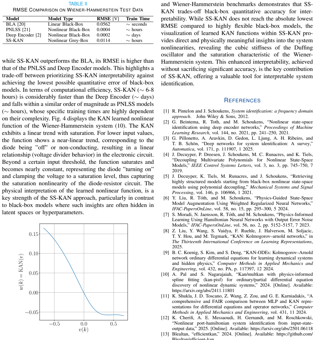
The central claim is that when a KAN is used to model only the nonlinear part of a state-space model, the trained univariate functions retain a readable relation to the physical nonlinearity. For the two-state Silverbox model, $\operatorname{KAN}_f$ for the velocity update, plotted against position with velocity and input fixed, is nearly $y \approx -996x^3 + 12.8x^2 - 24.6x - 0.115$; the cubic term carries the Duffing stiffness and a small quadratic term reflects a secondary effect known in the physical realization. For the Wiener-Hammerstein system, the learned KAN that sits between the two linear blocks forms a linear ramp that saturates, directly matching the diode-resistor behavior. In both cases the authors conclude that SS-KAN reveals system nonlinearities at the cost of accuracy relative to state-of-the-art black-box models, with test RMSEs of $0.0039\,\mathrm{V}$ and $0.0114\,\mathrm{V}$ on the two benchmarks.
Load-bearing premise
The load-bearing premise is that the trained state variables keep their physical meaning (position and velocity in the Silverbox case), so a univariate plot of the KAN with the other inputs fixed is a plot of the physical nonlinearity rather than of some mixed coordinate.
Editorial extensions
If this is right
- On the Silverbox benchmark, the learned velocity-state update is dominated by a cubic term, so a practitioner can read the Duffing stiffness off the model without knowing the equations in advance.
- On the Wiener-Hammerstein benchmark, the recovered intermediate function is linear with saturation, so the diode-resistor nonlinearity is visible even though the internal states are never measured.
- SS-KAN reaches test RMSEs of $0.0039\,\mathrm{V}$ and $0.0114\,\mathrm{V}$ on the two benchmarks, roughly an order of magnitude better than the best linear approximation but worse than the polynomial and deep-encoder nonlinear baselines.
- Training is practical, taking about an hour on the Silverbox case and six to eight hours on the Wiener-Hammerstein case on laptop-class hardware, versus multi-day deep-encoder training.
- The sparsity penalty plus one-at-a-time plotting identifies which input state drives the nonlinearity and shows the other directions contribute negligibly.
Reading between the lines
- The interpretability reading is coordinate-dependent in a way the paper does not formally settle: a similarity transformation of the state-space model leaves input-output behavior identical but would mix the KAN inputs, so a visible cubic curve could be tied to the chosen coordinate convention rather than to the physical displacement.
- A robustness test would be to retrain SS-KAN from several different near-identity linear initializations on the same Silverbox data; if the cubic curve consistently lands in the same state-update slot, the physical reading is much stronger.
- The same construction should transfer to other identifiable structural nonlinearities, such as Coulomb friction, backlash, or piecewise-linear stiffness, and the recovered univariate shapes could be compared against those known nonlinear maps.
- The paper sets $\operatorname{KAN}_g$ to zero for Silverbox; keeping it active would let SS-KAN expose sensor or output-mapping nonlinearities as well, with a second set of visualizable curves.
Signed reviews
Editorial analysis
A structured set of objections, weighed in public.
Referee Report
Summary. The paper proposes State-Space Kolmogorov-Arnold Networks (SS-KAN), which embed KANs as additive residual functions in a discrete-time state-space model, jointly training the linear matrices (A,B,C,D) and the KAN weights with L1/L2 regularization. The method is evaluated on two benchmark problems: the Silverbox Duffing oscillator and the Wiener-Hammerstein circuit. The paper reports RMSE values against BLA, PNLSS, and Deep Encoder baselines, and interprets visualized KAN functions as revealing a cubic stiffness nonlinearity in Silverbox and a diode-resistor saturation nonlinearity in Wiener-Hammerstein. The central claim is that SS-KAN trades a modest amount of accuracy for enhanced interpretability via sparsity and direct visualization of univariate functions.
Significance. If the interpretability claim is established, SS-KAN is a useful grey-box architecture that combines a linear state-space core with flexible univariate nonlinearities, and the two public benchmark demonstrations are relevant to the nonlinear system identification community. The paper is honest about the possibility that states may not remain physical and explicitly flags the assumption rather than hiding it. Its strengths include the use of widely used benchmark datasets, a clear formulation of the cost function, and a training cost that is competitive with existing nonlinear state-space methods. However, the central scientific claim that the visualized functions correspond to physical nonlinearities is currently supported mainly by a post-hoc reading of two fitted surfaces, one of which is supported by an analysis that is explicitly omitted from the manuscript. The evidence therefore falls short of the paper's stated claim that SS-KAN 'reveals' the physical nonlinearities, rather than merely being consistent with them under an unverified coordinate assumption.
major comments (5)
- [Sec. IV-B, Eq. (5)] The cubic interpretation of Fig. 2 assumes that the trained state vector retains the physical meaning of position and velocity. The state-space realization in Eq. (5) is invariant under any invertible similarity transform x' = T x, with A' = T A T^{-1}, B' = T B, C' = C T^{-1}, and KAN_f'(x',u) = T KAN_f(T^{-1}x',u). Nothing in the cost function (7), the L1 penalty, or the close-to-identity initialization proves or tests that training selects the original coordinate system. The text in Sec. IV-B that 'the KAN preserves the function inputs without mixing' addresses mixing inside the KAN layer, not the state-space realization ambiguity. The authors should add a concrete test, for example comparing the identified state trajectories with measured physical states, checking the learned A against a discretized physical model, or showing that the cubic shape is preserved under allowable similarity transforms. Without such evidence, the apparent cubic function in Fig. 2 could be a coordinate artifact.
- [Sec. IV-B, Silverbox results] The sentence in Sec. IV-B describing the 'complementary analysis, omitted here' is a load-bearing piece of evidence: it is used to claim that varying the velocity state and the input produces negligible univariate functions, thereby supporting the conclusion that sparsity isolated the position state as the dominant nonlinear input. Since this analysis is not shown, and since it directly supports the central interpretability claim, it should be included as a figure or at least as a quantitative summary table. The current text asks the reader to accept the main conclusion on the basis of an unverifiable result.
- [Eqs. (5) and (7), Fig. 2] There is a non-identifiability between the linear part A and the linear components of KAN_f: any linear function of x can be represented either in A or in the linear terms of the B-splines, so the decomposition into 'residual linear dynamics' and 'nonlinear terms' is not unique. The polynomial fit y ≈ -996x^3 + 12.8x^2 - 24.6x - 0.115 includes a linear term and a quadratic term alongside the cubic term, and the interpretation of these extra terms as 'subtle dynamic effects' is post-hoc. The authors should demonstrate, for instance on simulated data where the true nonlinearity is known, that the optimized decomposition recovers the true cubic coefficient and does not merely fit an arbitrary polynomial in the chosen coordinate system.
- [Sec. V-A, Eq. (10)] The Wiener-Hammerstein model is strongly structured: the cascade form (10) is imposed a priori, and the linear matrices are initialized using Chebyshev filter information from the benchmark reference. Consequently, the learned saturation curve in Fig. 4 is partly a consequence of the imposed structure and initialization rather than a discovery from input-output data alone. The paper should state explicitly which components are assumed and which are learned, and it should include a sensitivity test, such as random or less informed linear initializations, to show that the saturation shape is robust rather than a side effect of the chosen initialization.
- [Tables I and II] The RMSE comparisons combine numbers from different publications with different test protocols, model classes, and training setups, and no variance or repeated-seed statistics are reported for SS-KAN. The 'at the cost of accuracy' claim in the abstract and conclusion is therefore less precise than it should be. The authors should either add same-protocol baseline runs for at least one standard method or explicitly state the comparability limitations of the literature-derived RMSE values.
minor comments (5)
- [Table I paragraph] There is a typo in 'Deep Enconder'; it should read 'Deep Encoder'.
- [Abstract] The first sentence 'While accurate, black-box system identification models lack interpretability of the underlying system dynamics' is a fragment; it should be rephrased, for example 'Although they are accurate, black-box system identification models lack interpretability...'.
- [Eq. (5)] The notation uses KAN_f and KAN_g as both the function names and their vector-valued outputs; using explicit composition notation, such as f(x(k),u(k)) ≈ KAN_f(x(k),u(k)), would make the equations clearer.
- [Sec. IV-A and V-A] Hyperparameters such as λ_L1 = λ_L2 = 10^{-4}, the 5-point grid, and the hidden layer sizes are stated without sensitivity analysis; since the interpretability conclusion depends on the sparsity level, a short discussion or small ablation of λ_L1 would strengthen the claim.
- [Fig. 2 caption] The y-axis label 'KANf(x(k), ˙x, u) Nonlinear Output' is ambiguous because KAN_f is vector-valued; the caption should state explicitly which component of the KAN output is being plotted for the position update and which for the velocity update.
Circularity Check
No significant circularity: SS-KAN fits public benchmarks and its interpretability evidence is a post-hoc reading of fitted functions, not a prediction forced by construction or by self-citation.
full rationale
The paper's derivation chain is not circular. The model equations (5) and (10) are direct architectural definitions, the cost function (7) is a standard data-fit objective, and the reported RMSE values are validated against independent public benchmarks (Silverbox, Wiener-Hammerstein) and external baselines. No equation is defined in terms of the claimed result: the cubic shape in Fig. 2 and the saturation shape in Fig. 4 are outputs of the trained KANs, not constraints or fitted parameters renamed as predictions. The paper explicitly frames these as learned functions that 'reveal system nonlinearities', which is a post-hoc interpretation of fitted model components rather than a prediction derived from the model's own assumptions; that distinction weakens the interpretability claim's force but is not circularity. The self-citations in Section III-C ([4], [5], [15]) provide background on decoupled state-space models and are not load-bearing: the paper argues from the architecture that KANs take state variables as direct inputs 'without mixing', and it hedges the physical-interpretability conclusion with 'under the assumption of a well-approximated nonlinearity'. That hedge is an unproven correctness assumption, not a circular step. Two passages deserve explicit flagging but do not raise the circularity score. First, Section IV-B describes a 'complementary analysis ... omitted here' that allegedly confirms negligible contributions from velocity and input; this is unverifiable, unreported evidence and weakens empirical support. Second, the central interpretability claim depends on learned states retaining physical coordinates (position and velocity), which state-space similarity invariance makes non-obvious; the paper does not prove this, citing it as an assumption. Both are correctness/evidence limitations, not cases where the result reduces to its own inputs by construction.
Assumptions & free parameters
free parameters (5)
- Regularization weights lambda_L1 and lambda_L2 =
1e-4 (both)
- Silverbox KAN grid size and architecture =
5-point grid, 2 layers, hidden size 2
- Wiener-Hammerstein KAN architecture =
2 layers, hidden size 15, dynamic grid update
- Learning rates and batch sizes =
1e-3, batch 64 (Silverbox); 1e-4 decaying, batch 2048 (Wiener-Hammerstein)
- Polynomial fit to learned KAN_f velocity update =
-996 x^3 + 12.8 x^2 - 24.6 x - 0.115
assumptions (5)
- standard math Kolmogorov-Arnold representation theorem
- domain assumption KAN architecture with chosen layers and grid can approximate residual nonlinearities f and g well enough
- ad hoc to paper State variables remain physically interpretable after training
- domain assumption Fixing other variables at their mean values and varying one input isolates that input's effect
- domain assumption Wiener-Hammerstein benchmark has a static nonlinearity between two linear blocks
Cite this review
Pith. "Pith review of State-Space Kolmogorov Arnold Networks for Interpretable Nonlinear System Identification." pith.science (2026). https://pith.science/paper/AWOBBNWG
@misc{pith2026250616392,
  author       = {Pith},
  title        = {Pith review of: State-Space Kolmogorov Arnold Networks for Interpretable Nonlinear System Identification},
  year         = {2026},
  howpublished = {\url{https://pith.science/paper/AWOBBNWG}},
  note         = {Machine review of arXiv:2506.16392}
}
read the original abstract
While accurate, black-box system identification models lack interpretability of the underlying system dynamics. This paper proposes State-Space Kolmogorov-Arnold Networks (SS-KAN) to address this challenge by integrating Kolmogorov-Arnold Networks within a state-space framework. The proposed model is validated on two benchmark systems: the Silverbox and the Wiener-Hammerstein benchmarks. Results show that SS-KAN provides enhanced interpretability due to sparsity-promoting regularization and the direct visualization of its learned univariate functions, which reveal system nonlinearities at the cost of accuracy when compared to state-of-the-art black-box models, highlighting SS-KAN as a promising approach for interpretable nonlinear system identification, balancing accuracy and interpretability of nonlinear system dynamics.
Figures


Reference graph
Works this paper leans on
-
[1]
R. Pintelon and J. Schoukens,System identification: a frequency domain approach. John Wiley & Sons, 2012
work page 2012
-
[2]
Nonlinear state-space identification using deep encoder networks,
G. Beintema, R. Toth, and M. Schoukens, “Nonlinear state-space identification using deep encoder networks,”Proceedings of Machine Learning Research, vol. 144, no. 2021, pp. 241–250, 2021
work page 2021
-
[3]
Deep networks for system identification: A survey,
G. Pillonetto, A. Aravkin, D. Gedon, L. Ljung, A. H. Ribeiro, and T. B. Sch ¨on, “Deep networks for system identification: A survey,” Automatica, vol. 171, p. 111907, 1 2025
work page 2025
-
[4]
Decoupling Multivariate Polynomials for Nonlinear State-Space Models,
J. Decuyper, P. Dreesen, J. Schoukens, M. C. Runacres, and K. Tiels, “Decoupling Multivariate Polynomials for Nonlinear State-Space Models,”IEEE Control Systems Letters, vol. 3, no. 3, pp. 745–750, 7 2019
work page 2019
-
[5]
J. Decuyper, K. Tiels, M. Runacres, and J. Schoukens, “Retrieving highly structured models starting from black-box nonlinear state-space models using polynomial decoupling,”Mechanical Systems and Signal Processing, vol. 146, p. 106966, 1 2021
work page 2021
-
[6]
Physics-Guided State-Space Model Augmentation Using Weighted Regularized Neural Networks,
Y . Liu, R. T ´oth, and M. Schoukens, “Physics-Guided State-Space Model Augmentation Using Weighted Regularized Neural Networks,” IFAC-PapersOnLine, vol. 58, no. 15, pp. 295–300, 5 2024
work page 2024
-
[7]
Physics-Informed Learning Using Hamiltonian Neural Networks with Output Error Noise Models,
S. Moradi, N. Jaensson, R. T ´oth, and M. Schoukens, “Physics-Informed Learning Using Hamiltonian Neural Networks with Output Error Noise Models,”IFAC-PapersOnLine, vol. 56, no. 2, pp. 5152–5157, 7 2023
work page 2023
-
[8]
KAN: Kolmogorov–arnold networks,
Z. Liu, Y . Wang, S. Vaidya, F. Ruehle, J. Halverson, M. Soljacic, T. Y . Hou, and M. Tegmark, “KAN: Kolmogorov–arnold networks,” in The Thirteenth International Conference on Learning Representations, 2025
work page 2025
Show all 21 references
-
[9]
KAN-ODEs: Kolmogorov–Arnold network ordinary differential equations for learning dynamical systems and hidden physics,
B. C. Koenig, S. Kim, and S. Deng, “KAN-ODEs: Kolmogorov–Arnold network ordinary differential equations for learning dynamical systems and hidden physics,”Computer Methods in Applied Mechanics and Engineering, vol. 432, no. PA, p. 117397, 12 2024
2024
-
[10]
Kan/multkan with physics-informed spline fitting (kan-pisf) for ordinary/partial differential equation discovery of nonlinear dynamic systems,
A. Pal and S. Nagarajaiah, “Kan/multkan with physics-informed spline fitting (kan-pisf) for ordinary/partial differential equation discovery of nonlinear dynamic systems,” 2024. [Online]. Available: https://arxiv.org/abs/2411.11801
2024 arXiv
-
[11]
A comprehensive and FAIR comparison between MLP and KAN repre- sentations for differential equations and operator networks,
K. Shukla, J. D. Toscano, Z. Wang, Z. Zou, and G. E. Karniadakis, “A comprehensive and FAIR comparison between MLP and KAN repre- sentations for differential equations and operator networks,”Computer Methods in Applied Mechanics and Engineering, vol. 431, 11 2024
2024
-
[12]
Nonlinear port-hamiltonian system identification from input-state- output data,
K. Cherifi, A. E. Messaoudi, H. Gernandt, and M. Roschkowski, “Nonlinear port-hamiltonian system identification from input-state- output data,” 2025. [Online]. Available: https://arxiv.org/abs/2501.06118
2025 arXiv
-
[13]
efficientkan,
Blealtan, “efficientkan,” 2024. [Online]. Available: https://github.com/ Blealtan/efficient-kan
2024
-
[14]
Decoupled Weight Decay Regularization,
I. Loshchilov and F. Hutter, “Decoupled Weight Decay Regularization,” inInternational Conference on Learning Representations, 2017
2017
-
[15]
Decoupling multivariate functions using a non-parametric Filtered CPD approach,
J. Decuyper, K. Tiels, S. Weiland, and J. Schoukens, “Decoupling multivariate functions using a non-parametric Filtered CPD approach,” IFAC-PapersOnLine, vol. 54, no. 7, pp. 451–456, 7 2021
2021
-
[16]
Identification of the Silverbox Benchmark Using Nonlinear State-Space Models,
A. Marconato, J. Sj ¨oberg, J. Suykens, and J. Schoukens, “Identification of the Silverbox Benchmark Using Nonlinear State-Space Models,” IFAC Proceedings Volumes, vol. 45, no. 16, pp. 632–637, 7 2012
2012
-
[17]
Nonlinear Benchmarks,
Schoukens, “Nonlinear Benchmarks,” 2024. [Online]. Available: https://github.com/MaartenSchoukens/nonlinear benchmarks
2024
-
[18]
Identification of nonlinear systems using Polynomial Nonlinear State Space models,
J. Paduart, L. Lauwers, J. Swevers, K. Smolders, J. Schoukens, and R. Pintelon, “Identification of nonlinear systems using Polynomial Nonlinear State Space models,”Automatica, vol. 46, no. 4, pp. 647–656, 2010
2010
-
[19]
Wiener-hammerstein bench- mark,
J. Schoukens, J. Suykens, and L. Ljung, “Wiener-hammerstein bench- mark,” in15th IFAC Symposium on System Identification (SYSID 2009), July 6-8, 2009, St. Malo, France, 2009
2009
-
[20]
Modelling of Wiener- Hammerstein Systems via the Best Linear Approximation,
L. Lauwers, R. Pintelon, and J. Schoukens, “Modelling of Wiener- Hammerstein Systems via the Best Linear Approximation,”IFAC Proceedings Volumes, vol. 42, no. 10, pp. 1098–1103, 2009
2009
-
[21]
Identification of a Wiener-Hammerstein system using the polynomial nonlinear state space approach,
J. Paduart, L. Lauwers, R. Pintelon, and J. Schoukens, “Identification of a Wiener-Hammerstein system using the polynomial nonlinear state space approach,”Control Engineering Practice, vol. 20, no. 11, pp. 1133–1139, 11 2012
2012
Reviewed August 15, 2026 · model on record in the stance chip above.
Discussion (0). Continue with ORCID to comment.