Choice of Scoring Rules for Indirect Elicitation of Properties with Parametric Assumptions

Chicago; Ian A. Kash (Department of Computer Science; Lingfang Hu; University of Illinois at Chicago; USA.)

REVIEW 3 major objections 5 minor 30 references

Choice of Scoring Rules for Indirect Elicitation of Properties with Parametric Assumptions

T0 review · 3 major / 5 minor · reviewed 2026-08-15 · deepseek-v4-flash

Challenge this review Re-run · record.json Download PDF Read on arXiv ↗ Review JSON

Pith's one-line read The paper claims that in two-dimensional indirect elicitation with a parametric model, the optimal scoring-rule weight is decided by a single global comparison of the model curve's slope with the slope of the target property's contour…

desk verdict New problem and a sound decomposition, but Theorem 6.3 overclaims: its proof hides a domain restriction that makes the 2-D optimality results false in natural cases. read the letter →

arxiv 2506.17880 v1 pith:GA2YKWIQ submitted 2025-06-22 cs.LG stat.MEstat.ML

Lingfang Hu , Ian A. Kash (Department of Computer Science , University of Illinois at Chicago , Chicago , USA.) This is my paper · ORCID

classification cs.LGstat.MEstat.ML

keywords properscoringrulesindirectelicitationparametricmodelestimationweightselectionvarianceaccuracy-rewardinglossesmonotonetrajectoriescomplexity

verification ladder T0 review T1 audit T2 compute T3 formal

The pith

A machine-rendered reading of the paper's core claim, the machinery that carries it, and where it could break.

The reading

People often want to forecast an indirect statistical quantity such as variance, which is not directly elicitable but can be obtained from directly elicitable subproperties like the first two moments. When the forecast is restricted to a parametric family, changing the weights in a weighted sum of proper scoring losses changes the fitted subproperties and hence the estimated target. This paper argues that in the two-subproperty case the whole effect is governed by one geometric comparison: the slope of the parametric model curve against the slope of the target property's contour lines. If that comparison keeps a fixed sign, the estimated target moves monotonically as the weight grows and the best weight is an extreme value (zero or infinity in the limit); if the slopes oppose, an interior best weight exists. The claim matters because it turns a seemingly arbitrary choice of scoring-rule weights into a checkable structural condition on the model and the target.

What carries the argument

The load-bearing object is the derivative comparison between the model curve $R(r_1)$ and the target-contour function $T(r_1;t_0)$, expressed by the sign of $R'(r_1)-T'(r_1;t_0)$ at their intersections. The proof route is a two-step decomposition: Lemma 5.1 shows that increasing a weight $c_1$ can only lower that sub-loss at the minimizer, and with accuracy-rewarding losses this makes the fitted subproperty move monotonically toward the true value along the model curve. Theorem 6.2 shows that the target link $t$ is monotone along the model curve if and only if the slope difference keeps a constant sign, provided the target contours are differentiable and monotone. Theorem 6.3 combines these into the exhaustive zero/infinity/interior prescription for $c_1^*$.

What would settle it

Build a two-subproperty example that satisfies every condition of Theorem 6.3 - accuracy-rewarding losses, a smooth strictly increasing model curve $R$, differentiable monotone contours $T$ with $0<R'(r_1)<T'(r_1;t_0)$ throughout - choose a true point $\hat r$ off the curve, numerically minimise $c_1L_1+c_2L_2$ over the model for a sweep of $c_1$, and check whether $\gamma(\theta^*_c)$ monotonically approaches $\Gamma(p)$ with $c_1^*=+\infty$; any interior optimum or non-monotone approach would show the theorem's conclusion fails under its own hypotheses.

Watch

Extended reading notes

Core claim

The central discovery, stated as Theorem 6.3, is that under its assumptions - a differentiable strictly monotone parametric model curve, differentiable monotone target contours, and accuracy-rewarding sub-losses - the two-subproperty weight-selection problem collapses into one global inequality. Write the parametric subproperty model as a curve $r_2=R(r_1)$ and write the level sets of the target link $t$ as $r_2=T(r_1;t_0)$. If $R'(r_1)$ and $T'(r_1;t_0)$ have the same sign everywhere and $R'(r_1)<T'(r_1;t_0)$, then increasing $c_1$ always moves the estimated target $\gamma(\theta^*_c(p))$ closer to the true $\Gamma(p)$, so the best weight is $c_1^*=+\infty$; the reverse inequality gives $c_1^*=0$. If the two derivatives have opposite signs everywhere, the estimate first moves closer and then farther away, giving $c_1^*\in(0,+\infty)$. The mechanism is a decomposition: increasing $c_1$ improves the estimate of $r_1$ monotonically, and the target changes monotonically along the model curve exactly when $R'(r_1)-T'(r_1;t_0)$ keeps one sign. Thus, under the theorem's conditions, the choice among weights is not a matter of taste but a structural property of the model curve relative to the target's contours.

Load-bearing premise

The argument rests on the assumption that, across the entire region the fitted trajectory can visit, the model curve keeps a consistently ordered slope relative to the target property's contour lines, and that those contours are differentiable and monotone; if that slope ordering reverses anywhere, the monotonicity and zero-or-infinity conclusions are not guaranteed.

Editorial extensions

If this is right

In any two-subproperty model meeting the theorem's conditions, the optimal weight can be read off from a global slope inequality, so the choice requires no numerical search over weights.
Equal or balanced weights are generally not optimal in the same-sign regimes: the best configuration discards one subproperty or concentrates all weight on it, so the common default of equal weights can be systematically inferior.
When the slope signs are opposite, a finite interior best weight exists, but the true target value may still be unreachable at that optimum, as the paper notes.
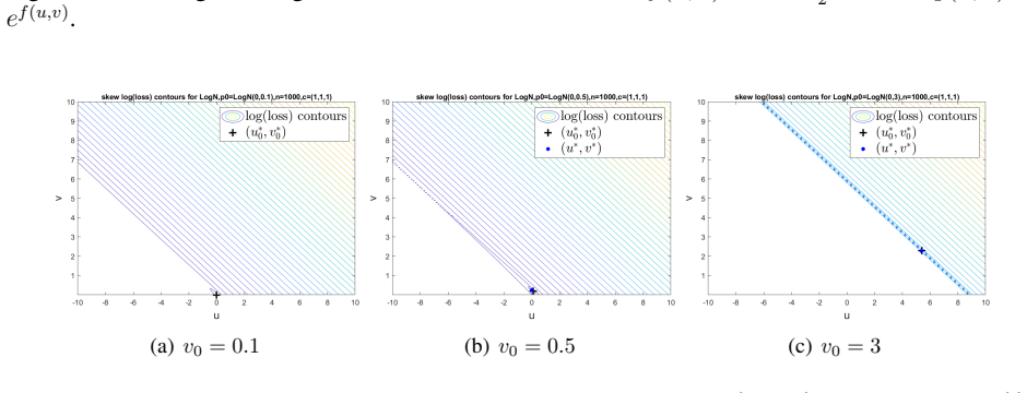
In higher dimensions the same monotonicity pattern holds for linear models, linear links, and linear trajectories, and nonlinear settings can be studied locally by linear approximation; this helps explain why simulations show monotonicity across different distribution families.

Reading between the lines

Editorial extensions of the paper, not claims the author makes directly.

A testable extension the paper does not run: construct a model where the slope ordering holds only in a local region and force the fitted trajectory to cross the sign-change boundary; the target-response curve should acquire a kink or reversal, which would delimit how far the global theorem extends.
The paper does not draw this conclusion, but the extreme-weight result suggests that a fully separable weighted loss is not a neutral tool for target estimation in the same-sign regimes: it wins by ignoring one of the subproperties entirely, so coupling the sublosses or choosing a different functional form might do better than any weight setting.
An implicit consequence for multi-objective loss design: the slope comparison can serve as a diagnostic for which objective to emphasize - put more weight on the coordinate along which the model curve cuts most steeply across the target's contours - which generalises beyond elicitation to any weighted composite loss.

Share X Bluesky LinkedIn Reddit HN

Signed reviews

No signed human review yet.

Editorial analysis

A structured set of objections, weighed in public.

Desk editor's note, referee report, and a circularity audit.

Desk Editor's Note

read the letter

Colleague,

The paper has a genuinely new problem and a theorem that is currently overclaimed. The two-step decomposition (Lemma 5.1 + Theorem 5.2) is clean and likely correct. But Theorem 6.3, the main 2-D payoff, has a hidden domain assumption that the proof calls "WLOG" and that is not WLOG at all. On reading the appendix, the proof assumes R^{-1}(rhat2) < rhat1 and uses points r_A and r_B as the c1=0 and c1=infinity endpoints. If rhat1 is outside the domain of R, r_B does not exist and the ordering arguments collapse. A concrete example: t(r)=r2-r1^2, R(r1)=r1+r1^2 on r1>0, and p=N(-1,0.5). Theorem 6.3(b) predicts c*_1=0, but direct minimization gives gamma(theta*) moving 0.823 -> 0.5 -> 0 as c1 increases, so the true c*_1 is finite. The theorem needs an explicit condition like rhat1 in the domain of R and R^{-1}(rhat2)

What is good: the problem statement is new, the simulations motivate the theory, and the decomposition into 'sub-property movement' and 'link monotonicity' is a useful way to think about weight selection. The paper is transparent that higher-dimensional theory is incomplete and that the renormalization trick is practical. The linear case (Theorem 7.2) is simple but fine.

The soft spots are proportional: the WLOG issue is load-bearing and makes Theorem 6.3 false as stated; the proof of Theorem 6.1 is a sketch with a domination argument; the simulations have no error bars and the renormalization is data-dependent, though disclosed. None of these sink the core idea, but they require a revision before the 2-D claims are trustworthy.

Who is this for? Researchers in property elicitation and scoring rules. It would get a serious referee, not a desk reject, because the problem is real and the counterexample points to a fix rather than a dead end. I would send it to review, but I would not cite the 2-D theorem in its current form.

Referee Report

3 major / 5 minor

Summary. The paper introduces the problem of choosing weights in a fully separable weighted sum of proper loss functions for indirect elicitation of a target property under a parametric model. For a target Gamma(p)=t(rhat(p)) with directly-elicited sub-properties rhat and a parametric sub-property curve r(theta), the minimizer theta*_c(p) depends on the weights c, and the paper studies how gamma(theta*_c(p)) changes with each c_i and which weight is best. The authors first report simulation evidence that weight trajectories are usually monotone and that optimal weights are often 0 or infinity. They then give an elementary decomposition (Theorem 5.2) into monotonicity of the sub-property trajectory and monotonicity of the link function, and provide 2-D sufficient conditions comparing the slope of the model curve R(r1) with the slope of the target contours T(r1;t0) (Theorem 6.3). For higher dimensions they prove a slice-wise monotonicity condition for the trajectory (Theorem 7.1) and treat linear cases (Theorem 7.2). The variance and skewness simulation studies are used to support the claimed empirical pattern.

Significance. If the main results were correct as stated, the paper would make a novel contribution to the sparse literature on choosing among proper scoring rules: it identifies a concrete geometric condition under which weight choice in indirect elicitation is determined by a slope comparison between the model curve and the target contour. The decomposition in Section 5 is elegant and potentially reusable, and the observation that boundary weights are often optimal is practically relevant. The paper is also commendably explicit about several limitations, including the incompleteness of the higher-dimensional theory and the assumed linearity of high-dimensional trajectories. However, the central 2-D theorem is stated for all p but its proof requires domain restrictions that are not part of the assumptions; this is a load-bearing gap rather than a presentational issue.

major comments (3)

[Appendix B, proof of Theorem 6.3] The proof uses 'Without loss of generality, assume that R^{-1}(rhat_2)<rhat_1' and then defines the endpoints r_A=(R^{-1}(rhat_2), rhat_2) and r_B=(rhat_1, R(rhat_1)) as the points reached as c1 approaches 0 and infinity. This is not WLOG: the assumptions of Theorem 6.3 do not imply that rhat_1 lies in the domain of R or that rhat_2 lies in the range of R, and they do not imply the required ordering. Since Problem 1 explicitly allows rhat outside R_Theta, the theorem's claim 'for all p' is unsupported. A concrete counterexample is t(r)=r2-r1^2, R(r1)=r1+r1^2 on r1>0, and p=N(-1,0.5), giving rhat=(-1,1.5). Here R'(r1)=1+2r1 > 2r1 = T'(r1;t0), so case (b) would predict c*_1=0, but minimizing c1(theta+1)^2 + (theta^2+theta-1.5)^2 over theta>0 gives gamma(theta*_0)≈0.823, gamma(theta*_1)≈0.5, and gamma(theta*_infinity)≈0, so the best weight is finite and close to 1. The theorem needs an explicit condition such as rhat_1 in the domain of R and R^{-1}(rhat_2)<rhat_1, or the statement must be restricted to p satisfying that condition.
[Section 6.2, Lemma B.1 and Theorem 6.2] The global monotone-contour assumption is not satisfied by the paper's own main example t(r)=r2-r1^2 on its full domain. Lemma B.1(2) requires the signs of partial derivatives to be unchanged over the whole space, but for this link function dt/dr1 = -2r1 changes sign, and the contour r2=r1^2+t0 is not a globally monotone function of r1. The paper applies the variance-link theory in Section 6.4 only on restricted positive-orthant regions, but Theorem 6.2 and Theorem 6.3 are stated with 'for all r1 and t0' and 'over the whole space.' This mismatch means the 'for all p' formulation of the 2-D result is not justified by the assumptions. The authors should either state the domain restriction explicitly in the theorems or reformulate the monotone-contour condition on the relevant domain of the model curve.
[Section 7.1 and Appendix D.1, Theorem 7.1] The induction proof of Theorem 7.1 rests on the claim that the intercepts epsilon'_k(r'_j) of each slice keep the same sign as epsilon_k for all r'_j below the axis intersection. This is the crux of the induction step, but the proof only says 'We can verify' and does not provide the verification. Given that the slice is merely strictly monotone, the sign preservation is not immediate and may require additional assumptions about how the slices vary with r'_j. The higher-dimensional condition (A) is therefore not fully proven as written. The later linear-case theorem (Theorem 7.2) also assumes linearity of the trajectories T_ci(p), which the paper explicitly states is not known to follow from linearity of r(theta); this should be clearly labeled as a conditional result rather than a theorem about the linear model alone.

minor comments (5)

[Section 3, Problem 1] The statement 'the choice of sub-losses does not affect our observation and conclusions' is too strong: the theorems require sub-losses to be accuracy-rewarding, and the simulation evidence is limited to quadratic losses. A more guarded statement would be more accurate.
[Section 4] The sentence 'In fact, the setting of c_{-i} does not matter for our empirical observations and theoretical results' is contradicted for M>2 by Remark 3, which notes that the normalization argument only applies in the 2-D case. Please qualify this claim.
[Section 2.1] There is a duplicated word in the introduction: 'there has been been more and more publications' should read 'there have been more and more publications.'
[Definition 5.2] The definition of 'one-sided from \tilde r_i' introduces a new symbol \tilde r, but the subsequent theorems use \hat r(p). Please make the notation consistent and specify which r is meant in each result.
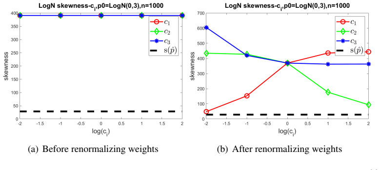
[Appendix F, Table 3] The reported skewness values for the log-normal examples are negative in the first block of Table 3, which is unexpected for log-normal models and mixtures of log-normals. Please check whether these are typos or whether a different sign convention is being used.

Circularity Check

0 steps flagged · score 0.0 of 10

No significant circularity: the paper's theoretical claims are derived from stated structural assumptions by calculus and optimization inequalities, not from fitted data or from a self-citation chain.

full rationale

Walking the derivation chain: the weighted loss is defined in Eq. (1), the estimator in Eq. (2), and Lemma 5.1 is a direct inequality consequence of optimality. Theorem 6.1 uses accuracy-rewarding sub-losses plus strict monotonicity of the model curve to constrain the possible region of r(theta*_c); this is a geometric argument, not a restatement of the conclusion. Lemma B.1 and Lemma B.2 relate monotonicity of t along R(r1) to the sign of R'(r1) - T'(r1; t0) via elementary calculus (Eqs. (3)-(4)), and Theorem 6.2/6.3 then combine those lemmas with Corollary B.2.1. None of these steps substitutes a fitted parameter for the claimed prediction: the derivative conditions are stated assumptions, not quantities fit to the simulated Gamma-ci curves. The simulations in Section 4 are explicitly exploratory, and the weight-renormalization trick in Remark 4/Appendix G is disclosed as a numerical device and stated not to affect the theoretical analysis. Citations such as Frongillo and Kash 2021 are background references on elicitation complexity and are not load-bearing for the paper's theorems. Possible domain restrictions in Theorem 6.3 (e.g., the 'without loss of generality' assumption R^{-1}(rhat2) < rhat1, or global monotonicity of contours) are correctness or robustness concerns, not circularity: if those assumptions fail the theorem may be false or need qualification, but the theorem is not equivalent to its inputs by construction.

Assumptions & free parameters 1 free parameters · 7 assumptions · 0 invented entities

The central claim rests on a series of assumptions about the loss functions, the parametric model, and the link function. In the theory, no constants are fitted from data; the only data-dependent quantity in the experimental protocol is the renormalization base k. The axioms are the load-bearing conditions that make the monotonicity theorems go through; several of them are global in scope while the applications check them only locally.

free parameters (1)

Weight renormalization base k_i = k_i = r_hat_2(p_hat) for skewness simulations
The authors renormalize weights by dividing by k_i = r_hat_2(p_hat) to mitigate optimization difficulties caused by dominant sub-losses. This data-dependent choice affects the reported Gamma_ci curves and the apparent best weights, and it is not derived from the theory.

assumptions (7)

domain assumption Sub-losses are accuracy-rewarding, a condition strictly stronger than strict properness.
Used throughout (Definition 2.4, Theorem 5.2, Theorem 6.1) to turn 'coordinate-wise closer to r_hat' into 'lower loss'.
domain assumption Optimizers theta*_c(p) exist for all p and c.
Assumed in Problem 1 and in all theorems; guarantees the object of study is well-defined.
ad hoc to paper The parametric sub-property model satisfies dim(Theta)=dim(R_Theta)=M-1.
Remark 1 states this is what makes the problem non-trivial; if the model were flexible enough to fit r_hat exactly, the choice of weights would not matter.
domain assumption In 2-D, r(theta) is a strictly monotone differentiable curve r2=R(r1).
Sufficient for condition (A) in Theorem 6.1; Appendix C argues more general curves can be decomposed into monotone pieces, but the formal theory relies on strict monotonicity.
domain assumption The link function t is continuous, partially differentiable, and all non-empty contours T(r1;t0) are differentiable and monotone.
Required by Theorem 6.2 and Lemmas B.1/B.2; this fails globally for t = r2 - r1^2, so the theorem is applied only on restriction to the positive orthant without explicit statement.
ad hoc to paper For M>2, trajectories T_ci(p) are assumed linear in Theorem 7.2, and slices of r(theta) are strictly monotone in Theorem 7.1.
The higher-dimensional theory is a linear special case; the paper itself acknowledges in Section 9 that the theory is incomplete for general high-dimensional settings.
domain assumption In simulations, p0 is chosen from the Gaussian family because tested models approximate Gaussian cases, and 1000 samples with a random seed are used.
This is an experimental design choice, not an axiom of the theory, but it shapes the empirical claims about monotonicity and best weights.

how reviews work

0 comments

Cite this review

Pith. "Pith review of Choice of Scoring Rules for Indirect Elicitation of Properties with Parametric Assumptions." pith.science (2026). https://pith.science/paper/GA2YKWIQ

@misc{pith2026250617880,
  author       = {Pith},
  title        = {Pith review of: Choice of Scoring Rules for Indirect Elicitation of Properties with Parametric Assumptions},
  year         = {2026},
  howpublished = {\url{https://pith.science/paper/GA2YKWIQ}},
  note         = {Machine review of arXiv:2506.17880}
}

read the original abstract

People are commonly interested in predicting a statistical property of a random event such as mean and variance. Proper scoring rules assess the quality of predictions and require that the expected score gets uniquely maximized at the precise prediction, in which case we call the score directly elicits the property. Previous research work has widely studied the existence and the characterization of proper scoring rules for different properties, but little literature discusses the choice of proper scoring rules for applications at hand. In this paper, we explore a novel task, the indirect elicitation of properties with parametric assumptions, where the target property is a function of several directly-elicitable sub-properties and the total score is a weighted sum of proper scoring rules for each sub-property. Because of the restriction to a parametric model class, different settings for the weights lead to different constrained optimal solutions. Our goal is to figure out how the choice of weights affects the estimation of the target property and which choice is the best. We start it with simulation studies and observe an interesting pattern: in most cases, the optimal estimation of the target property changes monotonically with the increase of each weight, and the best configuration of weights is often to set some weights as zero. To understand how it happens, we first establish the elementary theoretical framework and then provide deeper sufficient conditions for the case of two sub-properties and of more sub-properties respectively. The theory on 2-D cases perfectly interprets the experimental results. In higher-dimensional situations, we especially study the linear cases and suggest that more complex settings can be understood with locally mapping into linear situations or using linear approximations when the true values of sub-properties are close enough to the parametric space.

Figures

Figures reproduced from arXiv: 2506.17880 by the authors.

**Figure 2.** The Γci curves for Γ = var(·) with different qθ and pˆ. 8 [PITH_FULL_IMAGE:figures/full_fig_p008_2.png] view at source ↗

**Figure 3.** The impossible area of r(θ ∗ c ) for all c with a strictly monotone RΘ in a 2-D space, marked with gray shading. Theorem 6.1 For Problem 1 with M = 2, suppose that θ ∗ c (p) exists for all p and c and all sublosses are accuracy-rewarding. If r(θ) characterizes a strictly monotone function r2 = R(r1) 7 , then Tci (p) is one-sided from rˆi(p) for each i and all c−i , that is, Tci (p) is in the same quadrant centered … view at source ↗

Figures from the paper (24 more)

**Figure 4.** Figure 4: Example illustrations for Theorem 6.3, where each sub-figure corresponds to each sub [PITH_FULL_IMAGE:figures/full_fig_p014_4.png]

**Figure 5.** Figure 5: The display of different types of model assumptions for [PITH_FULL_IMAGE:figures/full_fig_p015_5.png]

**Figure 6.** Figure 6: Illustrative examples in 3-D where RΘ is a surface and θ ∈ R 2 . assumption, non-trivially there would be three different intersections between RΘ and the three axes centered at rˆ(p). Define the intercept on each axis-ri by εi , and then the global coordinates of the …

**Figure 7.** Figure 7: The sub-property trajectory Tc1 (pˆ) for different qθ. The blue surface is the level set of Γ = skew(·) nearby each trajectory [PITH_FULL_IMAGE:figures/full_fig_p018_7.png]

**Figure 8.** Figure 8: The Γci curves for the cases of Γ = var(·) and qθ = P oisson(θ) and p0 = N(θ0, θ0) with different θ0. (a) θ0 = 1 (b) θ0 = 10 (c) θ0 = 100 [PITH_FULL_IMAGE:figures/full_fig_p023_8.png]

**Figure 9.** Figure 9: The Γci curves for the cases of Γ = var(·) and qθ = χ 2 (θ) and p0 = N(θ0, 2θ0) with different θ0. (a) θ0 = 0.01 (b) θ0 = 1 (c) θ0 = 100 [PITH_FULL_IMAGE:figures/full_fig_p023_9.png]

**Figure 10.** Figure 10: The Γci curves for the cases of Γ = var(·) and qθ = Exponential(1/θ) and p0 = N(θ0, θ2 0 ) with different θ0. 23 [PITH_FULL_IMAGE:figures/full_fig_p023_10.png]

**Figure 11.** Figure 11: The Γci curves for the cases of Γ = var(·) and qθ = Gamma(K, θ) and p0 = N(Kθ0, Kθ2 0 ) with different θ0. (a) θ0 = 0.1 (b) θ0 = 0.5 (c) θ0 = 0.9 [PITH_FULL_IMAGE:figures/full_fig_p024_11.png]

**Figure 12.** Figure 12: The Γci curves for the cases of Γ = var(·) and qθ = B(10, θ) and p0 = N(10θ0, 10θ0(1 − θ0)) with different θ0. Notice that the monotonicity directions of Γci for the same i are opposite for (a) and (c). 24 [PITH_FULL_IMAGE:figures/full_fig_p024_12.png]

**Figure 13.** Figure 13: The impossible area of r(θ ∗ c ) for all c with a general RΘ in a 2-D space, marked with gray shading. In Section 6.1, we have proved in Theorem 6.1 that a strictly monotone r(θ) in 2-D cases makes the possible area of r(θ ∗ c ) for all c intrinsically restricted to o…

**Figure 14.** Figure 14: The Γci curves for the cases of Γ = skew(·) and qθ = LogN(u, v2 ) with different p0. (a) qθ = LogLogistic (b) qθ = Gamma (c) qθ = Beta [PITH_FULL_IMAGE:figures/full_fig_p032_14.png]

**Figure 15.** Figure 15: The Γci curves for the cases of Γ = skew(·) with different qθ. As mentioned in Section 7.2, to relieve the issue of optimization difficulties, we need to remove the dominance of poorly-behaved sub-losses with renormalizing the weights in the way c˜ = c./k, where ./ re…

**Figure 16.** Figure 16: The Γci curves for the cases of Γ = skew(·) and qθ = LogLogistic(a, b) with different p0 = LogLogistic(1, b0). 32 [PITH_FULL_IMAGE:figures/full_fig_p032_16.png]

**Figure 17.** Figure 17: The Γci curves for the cases of Γ = skew(·), qθ = Gamma(a, b) or qθ = Beta(a, b) with different p0. Each sub-figure corresponds to a specific setting for the parameter values (a0, b0) of p0. 33 [PITH_FULL_IMAGE:figures/full_fig_p033_17.png]

**Figure 18.** Figure 18: The Γci curves with different initial points for the gradient descent algorithm. It shows that the numerical optimization algorithm is sensitive to the choice of the initial point for iterations. Here, Γ = skew(·), qθ = LogN(u, v2 ) with θ = (u, v), p0 = LogN(0, 1 2 )…

**Figure 19.** Figure 19: The contours of log(Lc˜) with c = (1, 1, 1). Here, Γ = skew(·), qθ = LogN(u, v2 ) with θ = (u, v), p0 = LogN(0, 3 2 ). (Notice that the vertical axis refers to v 2 instead of v itself.) The loss contours are plot based on the total loss values on the meshgrid of width…

**Figure 20.** Figure 20: The contours of the total loss Lc˜ with c = (1, 1, 1), and also other sub-losses. Here, Γ = skew(·), qθ = LogN(u, v2 ) with θ = (u, v), p0 = LogN(0, 3 2 ). (Notice that the vertical axis refers to v 2 instead of v itself.) The loss contours are plot based on the total…

**Figure 21.** Figure 21: The original images and also contours of functions [PITH_FULL_IMAGE:figures/full_fig_p037_21.png]

**Figure 22.** Figure 22: The contours of the total loss Lc˜ for different p0 with c = (1, 1, 1). Here, Γ = skew(·), qθ = LogN(u, v2 ) with θ = (u, v), p0 = LogN(0, v2 0 ). (Notice that the vertical axis refers to v 2 instead of v itself.) In the above example, the dominance of L3 is caused by…

**Figure 23.** Figure 23: The contours of the total loss Lc˜ with c = (1, 1, 1) and different settings for k. Here, Γ = skew(·), qθ = LogN(u, v2 ) with θ = (u, v2 ), p0 = LogN(0, 3 2 ). (Notice that the vertical axis refers to v 2 instead of v itself.) even helps Γci reach a value closer to th…

**Figure 24.** Figure 24: The Γci curves with different different settings of k. Here, Γ = skew(·), qθ = LogN(u, v2 ) with θ = (u, v), p0 = LogN(0, 3 2 ). The initial point θ ∗ 0 for the optimization algorithm is the minimizer of the total loss on a meshgrid generated around the global minimi…

**Figure 25.** Figure 25: The Γci curves with different settings for k for the cases of qθ = LogN(u, v2 ) and p0 = LogN(0, v2 0 ). Each row corresponds to a different value of v0. Here, Γ = skew(·). 41 [PITH_FULL_IMAGE:figures/full_fig_p041_25.png]

**Figure 26.** Figure 26: The Γci curves with different settings for k for the cases of qθ = LogN(u, v2 ) and p0 from different families. Each row corresponds to a different family of p0. Here, Γ = skew(·). 42 [PITH_FULL_IMAGE:figures/full_fig_p042_26.png]

**Figure 27.** Figure 27: The Γci curves with different settings for k for the cases of qθ = LogLogistic(a, b). Each row corresponds to a different parameter setting of b0 for p0 = LogLogistic(a0, b0). Here, Γ = skew(·). 43 [PITH_FULL_IMAGE:figures/full_fig_p043_27.png]

Review history (2 revisions) →

Discussion (0). Continue with ORCID to comment.

Reference graph

Works this paper leans on

30 extracted references · 22 canonical work pages

[1]

A characterization of scoring rules for linear properties

Jacob D Abernethy and Rafael M Frongillo. A characterization of scoring rules for linear properties. In Conference on Learning Theory, pages 27--1. JMLR Workshop and Conference Proceedings, 2012

work page 2012
[2]

Introduction to machine learning

Ethem Alpaydin. Introduction to machine learning. MIT press, 2020

work page 2020
[3]

Expected information as expected utility

Jos \'e M Bernardo. Expected information as expected utility. the Annals of Statistics, pages 686--690, 1979

work page 1979
[4]

Some comparisons among quadratic, spherical, and logarithmic scoring rules

J Eric Bickel. Some comparisons among quadratic, spherical, and logarithmic scoring rules. Decision Analysis, 4 0 (2): 0 49--65, 2007

work page 2007
[5]

Verification of forecasts expressed in terms of probability

Glenn W Brier. Verification of forecasts expressed in terms of probability. Monthly weather review, 78 0 (1): 0 1--3, 1950

1950
[6]

An overview of applications of proper scoring rules

Arthur Carvalho. An overview of applications of proper scoring rules. Decision Analysis, 13 0 (4): 0 223--242, 2016

work page 2016
[7]

Optimal scoring rule design under partial knowledge

Yiling Chen and Fang-Yi Yu. Optimal scoring rule design under partial knowledge. arXiv preprint arXiv:2107.07420, 2021

arXiv 2021
[8]

Beyond strictly proper scoring rules: The importance of being local

Hailiang Du. Beyond strictly proper scoring rules: The importance of being local. Weather and forecasting, 36 0 (2): 0 457--468, 2021

work page 2021

Show all 30 references

[9]

Local proper scoring rules

Werner Ehm and Tilmann Gneiting. Local proper scoring rules. Journal of Machine Learning Research, 6: 0 695--709, 2009

2009
[10]

Higher order elicitability and osband's principle

Tobias Fissler and Johanna F Ziegel. Higher order elicitability and osband's principle. The Annals of Statistics, 44 0 (4): 0 1680--1707, 2016

2016
[11]

Effective scoring rules for probabilistic forecasts

Daniel Friedman. Effective scoring rules for probabilistic forecasts. Management Science, 29 0 (4): 0 447--454, 1983

1983
[12]

Recent trends in information elicitation

Rafael Frongillo and Bo Waggoner. Recent trends in information elicitation. ACM SIGecom Exchanges, 22 0 (1): 0 122--134, 2024

2024
[13]

Elicitation complexity of statistical properties

Rafael M Frongillo and Ian A Kash. Elicitation complexity of statistical properties. Biometrika, 108 0 (4): 0 857--879, 2021

2021
[14]

Information, incentives, and goals in election forecasts

Andrew Gelman, Jessica Hullman, Christopher Wlezien, and George Elliott Morris. Information, incentives, and goals in election forecasts. Judgment and Decision Making, 15 0 (5): 0 863--880, 2020

2020
[15]

Making and evaluating point forecasts

Tilmann Gneiting. Making and evaluating point forecasts. Journal of the American Statistical Association, 106 0 (494): 0 746--762, 2011

2011
[16]

Strictly proper scoring rules, prediction, and estimation

Tilmann Gneiting and Adrian E Raftery. Strictly proper scoring rules, prediction, and estimation. Journal of the American statistical Association, 102 0 (477): 0 359--378, 2007

2007
[17]

Rational decisions

Irving John Good. Rational decisions. Journal of the Royal Statistical Society: Series B (Methodological), 14 0 (1): 0 107--114, 1952

1952
[18]

Optimal scoring rules for multi-dimensional effort

Jason D Hartline, Liren Shan, Yingkai Li, and Yifan Wu. Optimal scoring rules for multi-dimensional effort. In The Thirty Sixth Annual Conference on Learning Theory, pages 2624--2650. PMLR, 2023

2023
[19]

Tailored scoring rules for probabilities

David J Johnstone, Victor Richmond R Jose, and Robert L Winkler. Tailored scoring rules for probabilities. Decision Analysis, 8 0 (4): 0 256--268, 2011

2011
[20]

Eliciting properties of probability distributions

Nicolas S Lambert, David M Pennock, and Yoav Shoham. Eliciting properties of probability distributions. In Proceedings of the 9th ACM Conference on Electronic Commerce, pages 129--138, 2008

2008
[21]

Optimization of scoring rules

Yingkai Li, Jason D Hartline, Liren Shan, and Yifan Wu. Optimization of scoring rules. In Proceedings of the 23rd ACM Conference on Economics and Computation, pages 988--989, 2022

2022
[22]

Contrasting probabilistic scoring rules

Reason L Machete. Contrasting probabilistic scoring rules. Journal of Statistical Planning and Inference, 143 0 (10): 0 1781--1790, 2013

2013
[23]

Measures of the value of information

John McCarthy. Measures of the value of information. Proceedings of the National Academy of Sciences, 42 0 (9): 0 654--655, 1956

1956
[24]

Choosing a strictly proper scoring rule

Edgar C Merkle and Mark Steyvers. Choosing a strictly proper scoring rule. Decision Analysis, 10 0 (4): 0 292--304, 2013

2013
[25]

Providing Incentives for Better Cost Forecasting (Prediction, Uncertainty Elicitation)

Kent Harold Osband. Providing Incentives for Better Cost Forecasting (Prediction, Uncertainty Elicitation). University of California, Berkeley, 1985

1985
[26]

Philip Dawid, and Steffen Lauritzen

Matthew Parry, A. Philip Dawid, and Steffen Lauritzen. Proper local scoring rules . The Annals of Statistics, 40 0 (1): 0 561--592, 2012. doi:10.1214/12-AOS971. URL https://doi.org/10.1214/12-AOS971

2012 doi
[27]

Elicitation of personal probabilities and expectations

Leonard J Savage. Elicitation of personal probabilities and expectations. Journal of the American Statistical Association, 66 0 (336): 0 783--801, 1971

1971
[28]

A family of strictly proper scoring rules which are sensitive to distance

Carl-Axel S Sta \"e l von Holstein. A family of strictly proper scoring rules which are sensitive to distance. Journal of Applied Meteorology and Climatology, 9 0 (3): 0 360--364, 1970

1970
[29]

Elicitation and identification of properties

Ingo Steinwart, Chlo \'e Pasin, Robert Williamson, and Siyu Zhang. Elicitation and identification of properties. In Conference on Learning Theory, pages 482--526. PMLR, 2014

2014
[30]

Scoring rules and the evaluation of probabilities

RL Winkler. Scoring rules and the evaluation of probabilities. Test: An Official Journal of the Spanish Society of Statistics and Operations Research, 5 0 (1): 0 1--60, 1996

1996

Pith tools

Reviewed August 15, 2026 · model on record in the stance chip above.

[1] [1]

A characterization of scoring rules for linear properties

Jacob D Abernethy and Rafael M Frongillo. A characterization of scoring rules for linear properties. In Conference on Learning Theory, pages 27--1. JMLR Workshop and Conference Proceedings, 2012

work page 2012

[2] [2]

Introduction to machine learning

Ethem Alpaydin. Introduction to machine learning. MIT press, 2020

work page 2020

[3] [3]

Expected information as expected utility

Jos \'e M Bernardo. Expected information as expected utility. the Annals of Statistics, pages 686--690, 1979

work page 1979

[4] [4]

Some comparisons among quadratic, spherical, and logarithmic scoring rules

J Eric Bickel. Some comparisons among quadratic, spherical, and logarithmic scoring rules. Decision Analysis, 4 0 (2): 0 49--65, 2007

work page 2007

[5] [5]

Verification of forecasts expressed in terms of probability

Glenn W Brier. Verification of forecasts expressed in terms of probability. Monthly weather review, 78 0 (1): 0 1--3, 1950

1950

[6] [6]

An overview of applications of proper scoring rules

Arthur Carvalho. An overview of applications of proper scoring rules. Decision Analysis, 13 0 (4): 0 223--242, 2016

work page 2016

[7] [7]

Optimal scoring rule design under partial knowledge

Yiling Chen and Fang-Yi Yu. Optimal scoring rule design under partial knowledge. arXiv preprint arXiv:2107.07420, 2021

arXiv 2021

[8] [8]

Beyond strictly proper scoring rules: The importance of being local

Hailiang Du. Beyond strictly proper scoring rules: The importance of being local. Weather and forecasting, 36 0 (2): 0 457--468, 2021

work page 2021