REVIEW 4 major objections 7 minor 30 references
Leveraging Lightweight Generators for Memory Efficient Continual Learning
T0 review · 4 major / 7 minor · reviewed 2026-08-15 · deepseek-v4-flash
Pith's one-line read The paper claims that replacing stored raw images with tiny SVD-based generators in replay-based continual learning methods can match or beat raw-sample memory at the same byte budget on low-complexity image tasks.
desk verdict A zero-training SVD replay generator that shows real gains on simple image domains, but the memory-matched baselines are confounded by 20x more fitting data and an unreported replay size n. read the letter →
The pith
A machine-rendered reading of the paper's core claim, the machinery that carries it, and where it could break.
The reading
What carries the argument
The central object is the lightweight SVD generator: for each task and class, a truncated singular value decomposition of the flattened image matrix yields $U_r$ (the top $r$ principal components), and the mean and covariance of the projected coefficients $V_h^r$, scaled by the singular values $S_r$; a synthetic sample is produced by drawing a random latent vector from the multivariate normal defined by those statistics and computing $U_r$ times that vector. This replaces the raw-sample episodic memory with a compact generative model that requires no training and costs $O(s)$ time to fit, and its memory footprint is $P\cdot r + r^2 + r$ entries per class.
What would settle it
Run the SVD-generator variant with the generator fitted on only 51 samples per class (matching the raw A-GEM and ER memory budget) and compare against the raw baseline storing 51 samples; if the accuracy advantage disappears, the reported gains are due to the larger fitting sample, not to compression.
Extended reading notes
Core claim
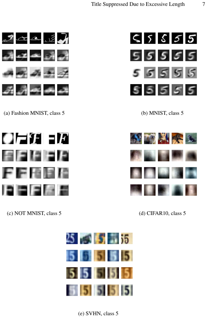
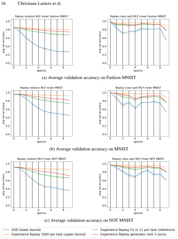
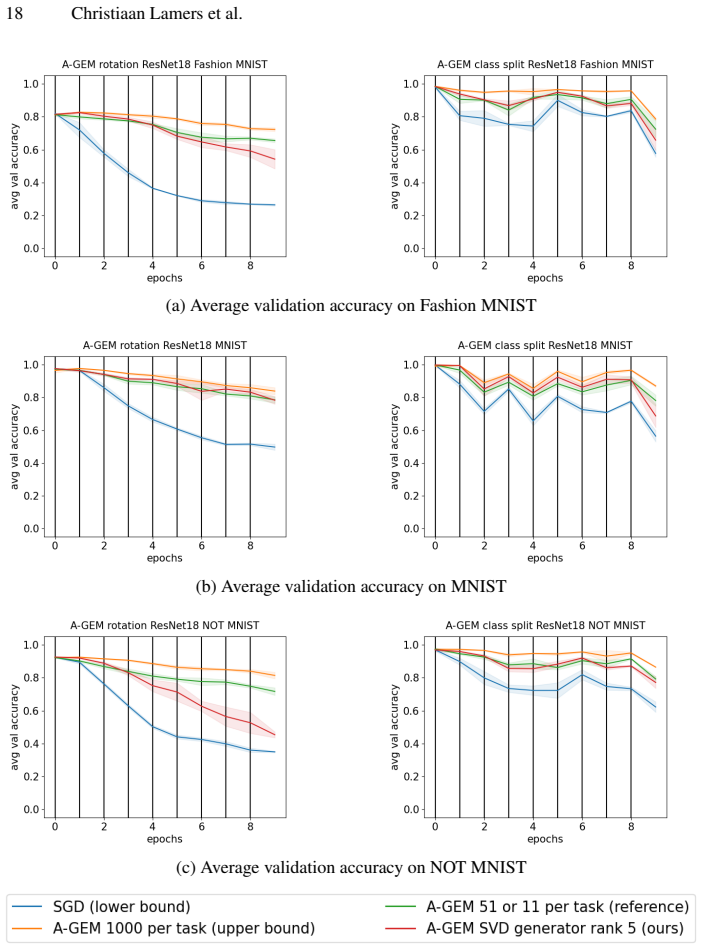
The central claim is that a truncated-SVD-based generator, fitted in linear time to the 1000 samples available per task and class, can serve as the episodic memory of A-GEM and Experience Replay and produce higher average validation accuracy than storing the equivalent number of raw samples (51 for rotation tasks, 11 for class-split tasks) in the same memory budget. The generator stores only the rank-truncated U matrix, the scaled mean, and the scaled covariance of the V-h matrix, and synthesizes samples by drawing a latent vector from a multivariate normal and multiplying by U. On MLP and MLP-mixer architectures, the method significantly outperforms the memory-matched raw baselines on Fashion-MNIST, MNIST, NOT-MNIST, and SVHN, while on ResNet18 it is at best on par, which the authors attribute to SVD capturing global rather than local patterns. On CIFAR10, a more complex dataset, the advantage shrinks or reverses unless the rank is raised to 80.
Load-bearing premise
The central comparison assumes that letting the generator fit on all 1000 samples available for a task while the memory-matched raw baseline stores only 51 or 11 randomly selected samples is a fair test of memory efficiency; if the accuracy gain comes mostly from the generator exploiting about 20 times more data during fitting, the claim that the compressed representation itself is the cause is not established.
Editorial extensions
If this is right
- Memory-matched replay now has a cheaper alternative: at the same byte budget, a rank-5 generator can outperform storing 51 raw samples on low-complexity datasets.
- The method drops into any rehearsal-based continual learning algorithm, not just A-GEM and ER, since the generator can be queried for arbitrary synthetic samples.
- On architectures that depend on local patterns (ResNet18), the generator provides no benefit, pointing to a mismatch between SVD's global components and convolutional features.
- Raising the rank to 80 recovers some of the advantage on CIFAR10 class-split tasks, indicating the compression-artifact tradeoff can be tuned per dataset.
- Because the generator fitting is a single linear-time SVD, the method adds almost no compute to the continual learning loop, unlike generative replay with VAEs or GANs.
Reading between the lines
- A fair test of compression would fit the generator on the same 51 or 11 samples the raw baseline stores; if the advantage disappears, the reported gains largely reflect access to 1000 samples during fitting rather than the SVD representation itself.
- The same truncated-SVD strategy could be applied to other memory-limited settings such as federated learning or on-device replay, where storing a few components per class may be cheaper than storing any raw images.
- The failure on ResNet18 suggests a testable extension: applying SVD to mid-layer feature maps rather than raw pixels might produce generators that capture the local patterns convolutional networks rely on.
- The linear-subspace assumption behind the generator—that each class's variation lives near a low-rank linear manifold—could be tested by measuring reconstruction error as a function of rank on a given dataset, which would predict when the method will work.
Signed reviews
Editorial analysis
A structured set of objections, weighed in public.
Referee Report
Summary. The paper proposes replacing the episodic memory of replay-based continual learning methods (A-GEM and Experience Replay) with lightweight generators based on truncated Singular Value Decomposition. For each task and class, the method fits an SVD on s=1000 randomly selected samples, stores only the top-r principal components U_r together with the scaled mean and covariance of the latent coefficients V_h, and generates synthetic replay samples by drawing from a multivariate normal in the latent space. The authors evaluate on Domain-IL rotation and class-split protocols across five datasets and three architectures, comparing against SGD, A-GEM/ER with 1000 stored samples per task, and A-GEM/ER with memory-matched budgets of 51 or 11 raw samples per task. The central claim is that, at equal memory, the SVD generator outperforms memory-matched raw-sample replay on low-complexity datasets and MLP-style architectures, while the authors honestly report that the advantage disappears or reverses on ResNet18 and CIFAR10.
Significance. If the central empirical claim holds, the paper offers a refreshingly simple and training-free alternative to generative replay with VAEs or GANs: a single linear-time SVD fit replaces stored raw samples, and the compression factor is explicit and easy to compute. The paper is transparent about scope, reporting negative results on convolutional architectures and on CIFAR10, and the method description is complete enough to be reimplemented. The main weakness is that the headline memory-matched comparison is confounded by unequal data access during memory construction, and several experimental parameters (notably the replay count n and storage precision) are not reported. These issues do not invalidate the idea but they do mean the paper's central claim is not yet established; the contribution would be strengthened substantially by the control experiments and reporting changes described below.
major comments (4)
- [Section 3.5 / Algorithms 1-3] The headline comparison is not memory-fair in terms of data access. The SVD generator is fitted on s=1000 samples per task, while the 'memory equivalent' A-GEM/ER baselines store only 51 (rotation) or 11 (class split) randomly selected raw samples. Random selection ignores the other ~950 samples, so the reported gains could come from the generator seeing 20-90x more data during memory construction rather than from the SVD representation itself. The A-GEM/ER 1000 upper bound does not control for this. To support the claim that compression is the cause of the improvement, add baselines that use the full 1000 samples to select the stored 51/11 (e.g., herding, k-means centers, or other coreset selection) and report whether the advantage persists.
- [Algorithms 1 and 2 / Section 3.5] The number n of generated samples used per replay step is never reported or discussed. n is a free parameter that determines the replay batch size and, in A-GEM, the quality of the reference gradient; if it differs from the baseline replay batch size, the comparison conflates storage efficiency with replay diversity. Please report n for every experiment and either match the per-step replay data count between the generator and raw-sample baselines or justify the discrepancy.
- [Section 3.4 / Eq. (1)] The compression factor counts scalar entries (P*r + r^2 + r) and compares them with raw pixels, without specifying numeric precision. If the stored SVD components are 32-bit floats and raw images are 8-bit uint8, the byte-level memory of the generator is about 4x larger than the formula implies, which would change the matched baseline from 51/11 samples to roughly 201/40 samples in the rotation/class-split settings. State the storage format (float16/float32/quantized) and report byte-level memory, or justify the entry-based convention with reference to the exact implementations used.
- [Section 3.6 / Tables 1-3] The primary reported number is accuracy averaged over all training epochs, whereas the standard continual-learning metric is average accuracy after each task (or at the end of the full sequence). Epoch-averaged accuracy can be high for a method that learns quickly and then forgets, so it does not directly measure forgetting. Please report final average accuracy after each task as the primary metric, with the epoch-averaged curves as secondary, and re-run the significance tests on the final values.
minor comments (7)
- [Section 3.5] The choice of rank r=5 and sample count s=1000 is justified only by 'satisfactory results in our early experiments'; describe the selection protocol or provide an ablation over r and s so that the reader can assess sensitivity to these free parameters.
- [Algorithm 3 / Section 3.2] The expression cov <- (Covariance(Vh) * S)^T * S is ambiguous because S is described as a vector; define S_r as a diagonal matrix and align the equation with the text's description of scaling the covariance on both axes.
- [Section 3.2] The abbreviation 'GANN' should be 'GAN'.
- [Section 4] In the discussion of Table 2, 'the it is on par with the ER 51 / 11 experiment' should read 'it is on par with the ER 51 / 11 experiment'.
- [Section 4] The sentence 'The generated images from SVHN (Figure 3d 4th row)' should refer to Figure 3e, since the SVHN panel is labeled (e).
- [Tables 1-3] The bold significance convention is unclear: the text does not state which pairwise comparisons are tested, and no multiple-comparison correction is applied across the many method/dataset/architecture combinations; please clarify the testing procedure.
- [References] Reference [24] for NOT-MNIST is incomplete; provide a URL and access date or a more formal citation.
Circularity Check
No significant circularity: the claimed gains are evaluated on held-out validation accuracy, not on any quantity fitted by the SVD generator.
full rationale
The paper's central comparison is empirical and self-contained. The lightweight generator is constructed by truncated SVD on per-class buffers of s=1000 task samples (Algorithms 1-3), with rank fixed at r=5 from early experiments. Its stored footprint is computed directly from the stored matrices in Equation 1, and the raw-sample baselines are assigned the same byte budget by rounding 1000/F samples per task. The evaluation metric in Equation 2 is average validation accuracy on unseen validation sets, so the reported advantage of A-GEM/ER with SVD generators over the memory-matched baselines is an external measurement, not an algebraic consequence of the construction. The fairness concern that the generator uses all 1000 fitting samples while the baseline stores only 51 or 11 random samples is a legitimate experimental-design confound, but it is not circularity: the baseline's accuracy is not derived from the generator's parameters, and the result could have gone either way. The single self-citation (Lamers et al. [9]) appears only as related work on K-means sample selection and is not load-bearing. Honest negative results on ResNet18 further show the method does not force the claimed outcome.
Assumptions & free parameters
free parameters (3)
- rank r =
5 (and 80 in later experiments)
- number of samples s per task for fitting =
1000
- number of generated samples n per replay =
not reported
assumptions (3)
- domain assumption Per-class data is approximately low-rank linear.
- domain assumption The SVD latent coefficients follow a multivariate Gaussian distribution.
- standard math Standard SVD and covariance estimation properties.
Cite this review
Pith. "Pith review of Leveraging Lightweight Generators for Memory Efficient Continual Learning." pith.science (2026). https://pith.science/paper/3UV34X46
@misc{pith2026250619692,
  author       = {Pith},
  title        = {Pith review of: Leveraging Lightweight Generators for Memory Efficient Continual Learning},
  year         = {2026},
  howpublished = {\url{https://pith.science/paper/3UV34X46}},
  note         = {Machine review of arXiv:2506.19692}
}
read the original abstract
Catastrophic forgetting can be trivially alleviated by keeping all data from previous tasks in memory. Therefore, minimizing the memory footprint while maximizing the amount of relevant information is crucial to the challenge of continual learning. This paper aims to decrease required memory for memory-based continuous learning algorithms. We explore the options of extracting a minimal amount of information, while maximally alleviating forgetting. We propose the usage of lightweight generators based on Singular Value Decomposition to enhance existing continual learning methods, such as A-GEM and Experience Replay. These generators need a minimal amount of memory while being maximally effective. They require no training time, just a single linear-time fitting step, and can capture a distribution effectively from a small number of data samples. Depending on the dataset and network architecture, our results show a significant increase in average accuracy compared to the original methods. Our method shows great potential in minimizing the memory footprint of memory-based continual learning algorithms.
Figures


Figures from the paper (24 more)







Reference graph
Works this paper leans on
-
[1]
Thrun,Lifelong Learning Algorithms, pp
S. Thrun,Lifelong Learning Algorithms, pp. 181–209. Boston, MA: Springer US, 1998
work page 1998
-
[2]
Continual lifelong learning with neural networks: A review,
G. I. Parisi, R. Kemker, J. L. Part, C. Kanan, and S. Wermter, “Continual lifelong learning with neural networks: A review,”Neural networks, vol. 113, pp. 54–71, 2019
2019
-
[3]
Three scenarios for continual learning,
G. M. Van de Ven and A. S. Tolias, “Three scenarios for continual learning,”arXiv preprint arXiv:1904.07734, 2019
arXiv 1904
-
[4]
The end of moore’s law: A new beginning for information technology,
T. N. Theis and H.-S. P. Wong, “The end of moore’s law: A new beginning for information technology,”Computing in science & engineering, vol. 19, no. 2, pp. 41–50, 2017
2017
-
[5]
Singular value decomposition and least squares solutions,
G. H. Golub and C. Reinsch, “Singular value decomposition and least squares solutions,” in Handbook for Automatic Computation: Volume II: Linear Algebra, pp. 134–151, Springer, 1971. Leveraging Lightweight Generators for Memory Efficient Continual Learning 19
work page 1971
-
[6]
A comprehensive survey of continual learning: theory, method and application,
L. Wang, X. Zhang, H. Su, and J. Zhu, “A comprehensive survey of continual learning: theory, method and application,”IEEE Transactions on Pattern Analysis and Machine Intel- ligence, 2024
work page 2024
-
[7]
Continual unsupervised representation learning,
D. Rao, F. Visin, A. Rusu, R. Pascanu, Y . W. Teh, and R. Hadsell, “Continual unsupervised representation learning,”Advances in neural information processing systems, vol. 32, 2019
2019
-
[8]
On tiny episodic memories in continual learning,
A. Chaudhry, M. Rohrbach, M. Elhoseiny, T. Ajanthan, P. K. Dokania, P. H. Torr, and M. Ranzato, “On tiny episodic memories in continual learning,”arXiv preprint arXiv:1902.10486, 2019
arXiv 1902
Show all 30 references
-
[9]
Clustering- based domain-incremental learning,
C. Lamers, R. Vidal, N. Belbachir, N. van Stein, T. B ¨aeck, and P. Giampouras, “Clustering- based domain-incremental learning,” inProceedings of the IEEE/CVF International Confer- ence on Computer Vision (ICCV) Workshops, pp. 3384–3392, October 2023
2023
-
[10]
Continual learning with deep generative replay,
H. Shin, J. K. Lee, J. Kim, and J. Kim, “Continual learning with deep generative replay,” Advances in neural information processing systems, vol. 30, 2017
2017
-
[11]
Generative replay with feedback connections as a general strategy for continual learning,
G. M. Van de Ven and A. S. Tolias, “Generative replay with feedback connections as a general strategy for continual learning,”arXiv preprint arXiv:1809.10635, 2018
2018 arXiv
-
[12]
The hippocampal formation as a hierarchical gener- ative model supporting generative replay and continual learning,
I. Stoianov, D. Maisto, and G. Pezzulo, “The hippocampal formation as a hierarchical gener- ative model supporting generative replay and continual learning,”Progress in Neurobiology, vol. 217, p. 102329, 2022
2022
-
[13]
Generative mod- els from the perspective of continual learning,
T. Lesort, H. Caselles-Dupr ´e, M. Garcia-Ortiz, A. Stoian, and D. Filliat, “Generative mod- els from the perspective of continual learning,” in2019 International Joint Conference on Neural Networks (IJCNN), pp. 1–8, IEEE, 2019
2019
-
[14]
Brain-inspired replay for continual learning with artificial neural networks,
G. M. Van de Ven, H. T. Siegelmann, and A. S. Tolias, “Brain-inspired replay for continual learning with artificial neural networks,”Nature communications, vol. 11, no. 1, p. 4069, 2020
2020
-
[15]
Reducing catastrophic forgetting in online class incre- mental learning using self-distillation,
K. Nagata, H. Ono, and K. Hotta, “Reducing catastrophic forgetting in online class incre- mental learning using self-distillation,”arXiv preprint arXiv:2409.11329, 2024
2024 arXiv
-
[16]
Orthogonal gradient descent for contin- ual learning,
M. Farajtabar, N. Azizan, A. Mott, and A. Li, “Orthogonal gradient descent for contin- ual learning,” inInternational Conference on Artificial Intelligence and Statistics, vol. 108, pp. 3762–3773, PMLR, 26–28 Aug 2020
2020
-
[17]
Gradient projection memory for continual learning,
G. Saha, I. Garg, and K. Roy, “Gradient projection memory for continual learning,”arXiv preprint arXiv:2103.09762, 2021
2021 arXiv
-
[18]
Efficient lifelong learning with a-gem,
A. Chaudhry, M. Ranzato, M. Rohrbach, and M. Elhoseiny, “Efficient lifelong learning with a-gem,”arXiv preprint arXiv:1812.00420, 2018
2018 arXiv
-
[19]
Experience replay for con- tinual learning,
D. Rolnick, A. Ahuja, J. Schwarz, T. Lillicrap, and G. Wayne, “Experience replay for con- tinual learning,”Advances in neural information processing systems, vol. 32, 2019
2019
-
[20]
Rethinking experience replay: a bag of tricks for continual learning,
P. Buzzega, M. Boschini, A. Porrello, and S. Calderara, “Rethinking experience replay: a bag of tricks for continual learning,” in2020 25th International Conference on Pattern Recogni- tion (ICPR), pp. 2180–2187, IEEE, 2021
2021
-
[21]
Tutorial: Complexity analysis of singular value decomposition and its variants,
X. Li, S. Wang, and Y . Cai, “Tutorial: Complexity analysis of singular value decomposition and its variants,”arXiv preprint arXiv:1906.12085, 2019
1906 arXiv
-
[22]
Fashion-mnist: a novel image dataset for benchmarking machine learning algorithms,
H. Xiao, K. Rasul, and R. V ollgraf, “Fashion-mnist: a novel image dataset for benchmarking machine learning algorithms,”arXiv preprint arXiv:1708.07747, 2017
2017 arXiv
-
[23]
The mnist database of handwritten digit images for machine learning research,
L. Deng, “The mnist database of handwritten digit images for machine learning research,” IEEE Signal Processing Magazine, vol. 29, no. 6, pp. 141–142, 2012
2012
-
[24]
Not mnist,
Y . Bulatov, “Not mnist,” 2011
2011
-
[25]
Cifar10,
A. Krizhevsky, V . Nair, and G. Hinton, “Cifar10,” 2009
2009
-
[26]
Reading digits in natural images with unsupervised feature learning,
Y . Netzer, T. Wang, A. Coates, A. Bissacco, B. Wu, A. Y . Ng,et al., “Reading digits in natural images with unsupervised feature learning,” inNIPS workshop on deep learning and unsupervised feature learning, vol. 2011, p. 7, Granada, Spain, 2011. 20 Christiaan Lamers et al
2011
-
[27]
Multilayer perceptron and neural networks,
M.-C. Popescu, V . E. Balas, L. Perescu-Popescu, and N. Mastorakis, “Multilayer perceptron and neural networks,”WSEAS Transactions on Circuits and Systems, vol. 8, no. 7, pp. 579– 588, 2009
2009
-
[28]
Multilayer perceptrons,
L. B. Almeida, “Multilayer perceptrons,” inHandbook of Neural Computation, pp. C1–2, CRC Press, 2020
2020
-
[29]
Mlp-mixer: An all-mlp architecture for vision,
I. Tolstikhin, N. Houlsby, A. Kolesnikov, L. Beyer, X. Zhai, T. Unterthiner, J. Yung, D. Key- sers, J. Uszkoreit, M. Lucic, and A. Dosovitskiy, “Mlp-mixer: An all-mlp architecture for vision,” 2021
2021
-
[30]
Deep residual learning for image recognition,
K. He, X. Zhang, S. Ren, and J. Sun, “Deep residual learning for image recognition,” in Proceedings of the IEEE conference on computer vision and pattern recognition, pp. 770– 778, 2016. Supplementary Material for: Leveraging Lightweight Generators for Memory Efficient Continu...
2016
Reviewed August 15, 2026 · model on record in the stance chip above.
Discussion (0). Continue with ORCID to comment.