REVIEW 3 major objections 6 minor 111 references
Line ratio identification of external photoevaporation
T0 review · 3 major / 6 minor · reviewed 2026-08-15 · deepseek-v4-flash
Pith's one-line read Emission-line ratios can identify external photoevaporation in stellar clusters without resolving the discs.
desk verdict A useful, honest new diagnostic atlas for external photoevaporation in unresolved proplyds, with the main caveat that the observability threshold omits nebular background; deserves peer review. read the letter →
The pith
A machine-rendered reading of the paper's core claim, the machinery that carries it, and where it could break.
The reading
What carries the argument
The load-bearing machinery is a one-dimensional model of the ionized proplyd wind: mass conservation with a constant sound-speed outflow gives n ∝ $r^{-2}$, a precomputed grid of mass-loss rates fixes the wind density from disc radius, host mass, FUV field, and surface density, and a photoionization code computes the radial emissivity profile of every line outside the hydrogen ionization front. Observables are obtained by integrating emissivity over a hemisphere, mimicking an unresolved proplyd. A line-selection metric combines the fractional slope of each line ratio with distance, its Spearman monotonicity, and its luminosity relative to Hα, producing sensitivity tables whose entries log10(f) give the factor by which a ratio changes between $10^{3}$ and $10^{6}$ G0. Three physical effects drive the strongest ratios: emission-volume shifts across the ionization fronts of different metals, critical-density effects that change whether emissivity scales as n or $n^{2}$, and temperature sensitivity of high-excitation lines.
What would settle it
Take spatially unresolved spectra of proplyd candidates in a distant massive cluster where the FUV field can be estimated, subtract the nebular background, and plot [SII] 6731 Å / [OIII] 5007 Å against projected distance from the O star; if the ratio does not rise monotonically by roughly two to three orders of magnitude as the FUV field drops from $10^{6}$ to $10^{3}$ G0, or the gradient disappears once [OI] 6300 Å and background emission are included, the central claim is falsified.
Extended reading notes
Core claim
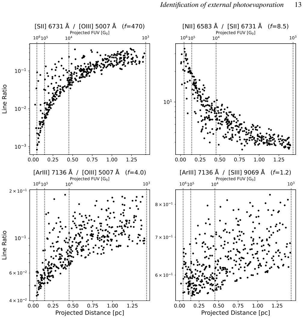
On the paper's own terms, the discovery is that external photoevaporation leaves a specific, monotonic fingerprint in spatially unresolved emission-line ratios. In the model, the ratio [SII] 6731 Å / [OIII] 5007 Å swings by a factor of 470 as the FUV field goes from $10^{6}$ to $10^{3}$ G0, because the volume where S II dominates shrinks roughly 25-fold and the volume where O III dominates shrinks roughly 7-fold relative to the hydrogen ionization front. Monte Carlo populations of proplyds with realistic stellar masses, disc radii, disc masses, and viewing geometries still show a clean spatial gradient for this ratio and for [NII] 6583 Å / [SII] 6731 Å (f = 8.5), while ratios with f ≈ 4 or 1.2 wash out. The paper therefore claims that line ratios with f ≳ 10 can identify ongoing external photoevaporation in stellar clusters even when individual proplyds are unresolvable, and that this conclusion barely depends on the spectral type of the ionizing star.
Load-bearing premise
The results assume that all chosen diagnostic lines come only from the ionized wind outside the hydrogen ionization front, ignoring emission from the photodissociation region, the disc, and the surrounding nebula.
Editorial extensions
If this is right
- Line ratios with f ≳ 10, led by [SII] 6731 Å / [OIII] 5007 Å, should show observable spatial gradients in unresolved cluster spectroscopy.
- The gradient shape is largely insensitive to whether the ionizing star is B0, O7, or O3, so the same diagnostic can be applied to clusters with different OB populations.
- The best diagnostic lines are predicted to lie in the optical and UV, with [OII] 3726 Å particularly promising for future blue-optical and UV facilities.
- The sensitivity tables provide a ready-made list of ratio pairs, letting observers choose the brightest and most sensitive tracers for their wavelength coverage.
- An initial test against five ONC proplyds shows the expected trend of [SII] 6731 Å / [OIII] 4959 Å increasing with projected distance, with one anomalous proplyd attributed to a jet and line-of-sight geometry.
Reading between the lines
- Beyond the paper, the same logic suggests a two-step survey strategy: use unresolved line-ratio gradients to identify clusters with ongoing external photoevaporation, then target those clusters with resolved follow-up spectroscopy.
- Because the model excludes emission from inside the ionization front, the practical diagnostic may be a composite that combines an ionized-wind ratio like [SII]/[OIII] with a PDR tracer such as [OI] 6300 Å to suppress contamination.
- A testable extension would be to search for these gradients in existing wide-field IFU data of known clusters, checking whether the ratio rises monotonically outward once nebular background lines are subtracted.
Signed reviews
Editorial analysis
A structured set of objections, weighed in public.
Referee Report
Summary. This paper presents a fast 1D model of emission lines from the ionized wind of externally photoevaporating protoplanetary discs. The wind density is assumed to follow n ∝ r^{-2} with a constant sound-speed velocity, the mass loss rate is taken from the FRIED grid, and CLOUDY is used to compute radial emissivity profiles. After benchmarking against VLT/MUSE observations of the ONC proplyd 177-341W, the authors run the model over FUV fields 10^3–10^6 G0, rank thousands of lines by a line-selection metric, and produce sensitivity tables for MUSE and broader wavelength ranges. They then perform Monte Carlo cluster simulations with projected distances, inclinations, and PDR obscuration, and argue that line ratios varying by f≳10 over the FUV range should show observable spatial gradients in unresolved cluster spectroscopy. The headline diagnostic is [SII] 6731 Å / [OIII] 5007 Å, which varies by a factor of 470 in the base model.
Significance. The proposed diagnostic addresses a real and timely observational need: external photoevaporation is currently studied mostly in resolved ONC proplyds, while more distant massive clusters require unresolved spectral diagnostics. The model is computationally efficient, and the sensitivity tables, data release, and use of public CLOUDY/FRIED codes make the work reproducible and immediately usable by the community. The physical interpretation in terms of ionization-front radii, critical densities, and temperature sensitivity provides a useful framework for understanding why certain ratios are sensitive to the FUV field. The predictions are falsifiable with existing and planned instruments. The paper is appropriately cautious about the simplicity of the wind model and the exclusion of interior-I-front emission in several places, although the observability analysis does not fully carry this caution through to the detectability claims.
major comments (3)
- [Section 4.3.1, Table 2] The detectability simulations in Section 4.3.1 include projection and inclination effects but omit nebular background emission, even though Section 1 acknowledges that high-UV environments are associated with substantial nebular emission. The benchmark in Table 2 shows that the model underpredicts [SII] 6716 relative to Hα by a factor of about 3.3 (Hα/[SII] observed 400 vs simulated 1300). Since [SII] 6731 is the numerator of the headline ratio [SII]/[OIII], any unresolved background with its own [SII]/[OIII] gradient will dilute or modify the predicted trend. The f≳10 threshold stated in Section 4.3.1 is therefore an internal model threshold, not a demonstrated detectability limit for real unresolved cluster spectroscopy. Please add a contaminant model, or otherwise quantify how the predicted gradients survive the level of background implied by the benchmark discrepancy.
- [Section 3.1, Table 2] The benchmark forces agreement by scaling the mass loss rate by a factor of 1.79 to match the Hα peak radius and by deriving extinction from the observed Hα/Hβ ratio. The Hα peak-position match is therefore enforced by construction. The factor-of-3 discrepancies in [SII] 6716 and [NII] 6583 line ratios show that the model is not calibrated for absolute line ratio levels. This is acceptable for trend predictions, but the paper should state clearly that the benchmark validates the ionization structure rather than the line-ratio normalization, and it should explain why the [SII]/[OIII] predictions are expected to be robust to a factor-of-3 level of contamination from processes not included in the model.
- [Section 4.1.3, Table 5] The observational test of the [SII] 6731 / [OIII] 4959 trend uses only five proplyds and shows very large scatter: 177-341W at 0.049 pc has a ratio of 0.0095, while 173-236 at 0.095 pc has 19. Even after excluding the anomalous 170-337, the implied change over 0.05 pc is far steeper than the base-case model trend in Figure 5. The paper should either provide a quantitative comparison with the model, including the expected Monte Carlo spread in mass loss rates and distances, or describe this as an illustrative anecdote rather than a 'preliminary trend' that supports the model.
minor comments (6)
- [Table 1] The surface density normalization is listed as Σau = 100 g/cm3, but surface density should be in units of g/cm^2; please correct the unit.
- [Section 4.2, Eq. (17)] The statement that r_m/r_IF 'always' increases when moving to larger distance (Y>1, X<1) does not follow from Eq. (17) in general, since X^{1/6}Y^{1/3} can be less than 1 if the mass loss rate falls steeply with distance. The plotted base-case results support the trend, but the 'always' claim should be replaced by a statement about the FRIED-grid dependence.
- [Section 2.3, Eqs. (4)-(6)] The notation for the optically thin limit, 'dτ(r)=0 for all r', is inconsistent with the definition of τ(x,y0) in Eq. (5); please clarify that the limit reduces the projected intensity integrals to volume integrals of j(r).
- [Section 5.4] The caveats list jets, bow shocks, tail emission, abundance variations, and multiple OB stars as additional noise sources, but do not explicitly list nebular background emission from the H II region itself, despite its prominence in the Introduction and its likely contribution to the benchmark [SII] discrepancy.
- [Section 4.1.1, Eqs. (9)-(10)] The line-selection measure RM uses an ad hoc weighting function h(x); the robustness of the selected line set to this choice of weighting is not tested. A brief sensitivity test, or at least a statement that the full tables are available for users to apply other metrics, would strengthen the methodology.
- [Section 5.3] The sentence 'Störzer & Hollenbach (1998); Ballabio et al. (2023) found that G ≳ 5000 G0 the [Oi] 6300 Å line luminosity rises significantly' is missing a word; it should read 'found that for G ≳ 5000 G0 ...'.
Circularity Check
No significant circularity: predicted line ratios are independent CLOUDY/FRIED outputs, not fitted to the trends they claim to diagnose.
full rationale
The derivation chain is: the FRIED grid supplies a mass-loss rate for the proplyd/UV-source parameters; mass conservation gives an n∝r^-2 wind density; CLOUDY performs the photoionization/radiative-transfer calculation and returns radial emissivities; line ratios are integrated volume luminosities. Section 3 benchmarks against the ONC proplyd 177-341W by rescaling the FRIED mass-loss rate by 1.79 so that the H-alpha intensity-peak radius matches the observed 82 au and by normalizing the H-alpha intensity, but those normalizations are not carried into the Section 4.1 base-case line-ratio predictions, and the observed line-ratio trends are never used as fitting constraints. The line-selection metric RM_ij in Section 4.1.1 ranks model outputs by sensitivity and luminosity; reporting the top-ranked ratios is a data-reduction/ranking step, not a circular derivation, and Sections 4.2.1-4.2.4 independently attribute the trends to ionization-front radii, critical densities, and temperature. The Monte Carlo observability study in Section 4.3 uses the same model plus projection, inclination, and PDR obscuration; it is an internal feasibility estimate with explicit caveats in Section 5.4, not a fitted quantity renamed as a prediction. The FRIED grid and MUSE observations are from overlapping author groups, but they are public, independently tested resources, and no uniqueness theorem or load-bearing self-citation forces the conclusions. The exclusion of [OI] 6300, PDR/interior emission, and nebular background is a completeness limitation correctly acknowledged in Sections 5.3 and 5.4, not a circular step.
Assumptions & free parameters
free parameters (5)
- Benchmark mass loss rate scaling factor =
1.79
- Surface density normalization Sigma_au =
100 g/cm^2 (representative)
- Extinction law parameters =
CCM89, R_V = 5.5, A(Halpha) from Halpha/Hbeta = 6.1
- Base-case proplyd parameters =
M_h = 0.7 M_sun, r_d = 50 au, i = 90 deg
- Monte Carlo sampling distributions =
uniform FUV 10^3 to 10^6 G0, uniform r_d 10 to 50 au, disc mass 10 to 50% M_max
assumptions (7)
- domain assumption The ionized wind starts at the hydrogen ionization front with constant velocity equal to the sound speed, so n is proportional to r^-2 (Eq. 1).
- domain assumption All selected diagnostic lines originate in the ionized wind outside r_IF; emission from the PDR, disk, and neutral region is negligible for those lines.
- domain assumption CLOUDY with Orion abundances adequately predicts the ionization and temperature structure of proplyd winds.
- domain assumption FRIED mass loss rates are accurate for the sampled proplyd parameters.
- domain assumption For metal ionization fronts, the ionizing photon intensity is approximately constant, giving U_IF n_IF = U_m n_m (Section 4.2.1).
- domain assumption Cluster observability can be approximated by random isotropic viewing angles, projected distances, and binary PDR/disc obscuration.
- standard math Mass conservation for a spherical outflow and case B recombination balance (Eqs. 1 and 2).
Cite this review
Pith. "Pith review of Line ratio identification of external photoevaporation." pith.science (2026). https://pith.science/paper/CFKV3GVH
@misc{pith2026250619788,
  author       = {Pith},
  title        = {Pith review of: Line ratio identification of external photoevaporation},
  year         = {2026},
  howpublished = {\url{https://pith.science/paper/CFKV3GVH}},
  note         = {Machine review of arXiv:2506.19788}
}
abstract
External photoevaporation of protoplanetary discs, by massive O stars in stellar clusters, is thought to be a significant process in the evolution of a disc. It has been shown to result in significant mass loss and disc truncation, ultimately reducing the lifetime of the discs, and possibly affecting potential planet populations. It is a well-studied process in the Orion Nebula Cluster (ONC) where the cometary morphology of proplyds is spatially resolvable due to its proximity to Earth. However, we need to study external photoevaporation in additional stellar clusters to better understand its prevalence and significance more globally. Unfortunately, more massive stellar clusters where the majority of stars form are much farther away than the ONC. In these more distant clusters the proplyds are spatially unresolvable with current facilities, hence the cometary morphology is not a useful identification of external photoevaporation. Therefore, in order to identify and interpret external photoevaporation, the only observations we have are of spatially unresolved emission lines. To resolve this issue we have used the CLOUDY code to develop an approximate general model of the emission lines emanating from the hot ionized wind of a proplyd. We have used the model to determine which line ratios are most sensitive to the distance from an OB star, and found that the most sensitive line ratios vary by multiple orders of magnitude over an FUV field of between 10$^3$ G$_0$ to 10$^6$ G$_0$. By identifying spatial gradients of line ratios in stellar clusters, we can identify regions of ongoing external photoevaporation.
Figures


Figures from the paper (6 more)



Reference graph
Works this paper leans on
-
[1]
write newline
" write newline "" before.all 'output.state := FUNCTION fin.entry write newline FUNCTION new.block output.state before.all = 'skip after.block 'output.state := if FUNCTION new.sentence output.state after.block = 'skip output.state before.all = 'skip after.sentence 'output.state := if if FUNCTION not #0 #1 if FUNCTION and 'skip pop #0 if FUNCTION or pop #1...
-
[2]
Adams F. C., Hollenbach D., Laughlin G., Gorti U., 2004, @doi [ ] 10.1086/421989 , https://ui.adsabs.harvard.edu/abs/2004ApJ...611..360A 611, 360
doi:10.1086/421989 2004
-
[3]
Allen M., et al., 2025, @doi [The Open Journal of Astrophysics] 10.33232/001c.137538 , https://ui.adsabs.harvard.edu/abs/2025OJAp....8E..54A 8, 54
-
[4]
Anania R., Winter A. J., Rosotti G., Vioque M., Zari E., Pantaleoni Gonz \'a lez M., Testi L., 2025, @doi [ ] 10.1051/0004-6361/202453011 , https://ui.adsabs.harvard.edu/abs/2025A&A...695A..74A 695, A74
-
[5]
Aru M. L., et al., 2024a, @doi [ ] 10.1051/0004-6361/202349004 , https://ui.adsabs.harvard.edu/abs/2024A&A...687A..93A 687, A93
-
[6]
Aru M. L., et al., 2024b, @doi [ ] 10.1051/0004-6361/202451737 , https://ui.adsabs.harvard.edu/abs/2024A&A...692A.137A 692, A137
-
[7]
Bacon R., et al., 2010, in McLean I. S., Ramsay S. K., Takami H., eds, Society of Photo-Optical Instrumentation Engineers (SPIE) Conference Series Vol. 7735, Ground-based and Airborne Instrumentation for Astronomy III. p. 773508 ( @eprint arXiv 2211.16795 ), @doi 10.1117/12.856027
arXiv 2010
-
[8]
Ballabio G., Haworth T. J., Henney W. J., 2023, @doi [ ] 10.1093/mnras/stac3467 , https://ui.adsabs.harvard.edu/abs/2023MNRAS.518.5563B 518, 5563
Show all 111 references
-
[9]
P., et al., 2023, @doi [ ] 10.3847/1538-4357/ace901 , https://ui.adsabs.harvard.edu/abs/2023ApJ...954..127B 954, 127
Ballering N. P., et al., 2023, @doi [ ] 10.3847/1538-4357/ace901 , https://ui.adsabs.harvard.edu/abs/2023ApJ...954..127B 954, 127
2023 doi
-
[10]
R., McCaughrean M
Bally J., O'Dell C. R., McCaughrean M. J., 2000, @doi [ ] 10.1086/301385 , https://ui.adsabs.harvard.edu/abs/2000AJ....119.2919B 119, 2919
2000 doi
-
[11]
Bern \'e O., et al., 2022, @doi [ ] 10.1088/1538-3873/ac604c , https://ui.adsabs.harvard.edu/abs/2022PASP..134e4301B 134, 054301
2022 doi
-
[12]
Bern \'e O., et al., 2023, @doi [ ] 10.1038/s41586-023-06307-x , https://ui.adsabs.harvard.edu/abs/2023Natur.621...56B 621, 56
2023 doi
-
[13]
Bern \'e O., et al., 2024, @doi [Science] 10.1126/science.adh2861 , https://ui.adsabs.harvard.edu/abs/2024Sci...383..988B 383, 988
2024 doi
-
[14]
S., et al., 2021, @doi [ ] 10.3847/1538-4365/ac1ad4 , https://ui.adsabs.harvard.edu/abs/2021ApJS..257...16B 257, 16
Booth A. S., et al., 2021, @doi [ ] 10.3847/1538-4365/ac1ad4 , https://ui.adsabs.harvard.edu/abs/2021ApJS..257...16B 257, 16
2021 doi
-
[15]
D., Eisner J
Boyden R. D., Eisner J. A., 2020, @doi [ ] 10.3847/1538-4357/ab86b7 , https://ui.adsabs.harvard.edu/abs/2020ApJ...894...74B 894, 74
2020 doi
-
[16]
D., Eisner J
Boyden R. D., Eisner J. A., 2023, @doi [ ] 10.3847/1538-4357/acaf77 , https://ui.adsabs.harvard.edu/abs/2023ApJ...947....7B 947, 7
2023 doi
-
[17]
D., Eisner J
Boyden R. D., Eisner J. A., 2024, @doi [ ] 10.3847/1538-4357/ad3cd5 , https://ui.adsabs.harvard.edu/abs/2024ApJ...967..103B 967, 103
2024 doi
- [18]
-
[19]
R., et al., 2024, in Bryant J
Brandl B. R., et al., 2024, in Bryant J. J., Motohara K., Vernet J. R. D., eds, Society of Photo-Optical Instrumentation Engineers (SPIE) Conference Series Vol. 13096, Ground-based and Airborne Instrumentation for Astronomy X. p. 1309612, @doi 10.1117/12.3018975
2024 doi
-
[20]
A., Clayton G
Cardelli J. A., Clayton G. C., Mathis J. S., 1989, @doi [ ] 10.1086/167900 , https://ui.adsabs.harvard.edu/abs/1989ApJ...345..245C 345, 245
1989 doi
-
[21]
Chatzikos M., et al., 2023, @doi [ ] 10.22201/ia.01851101p.2023.59.02.12 , https://ui.adsabs.harvard.edu/abs/2023RMxAA..59..327C 59, 327
2023 doi
-
[22]
J., 2007, @doi [ ] 10.1111/j.1365-2966.2007.11547.x , https://ui.adsabs.harvard.edu/abs/2007MNRAS.376.1350C 376, 1350
Clarke C. J., 2007, @doi [ ] 10.1111/j.1365-2966.2007.11547.x , https://ui.adsabs.harvard.edu/abs/2007MNRAS.376.1350C 376, 1350
2007
-
[23]
Coleman G. A. L., Haworth T. J., 2022, @doi [ ] 10.1093/mnras/stac1513 , https://ui.adsabs.harvard.edu/abs/2022MNRAS.514.2315C 514, 2315
2022 doi
-
[24]
Concha-Ram \' rez F., Wilhelm M. J. C., Portegies Zwart S., Haworth T. J., 2019, @doi [ ] 10.1093/mnras/stz2973 , https://ui.adsabs.harvard.edu/abs/2019MNRAS.490.5678C 490, 5678
2019 doi
-
[25]
J., 2023, @doi [European Physical Journal Plus] 10.1140/epjp/s13360-022-03602-w , https://ui.adsabs.harvard.edu/abs/2023EPJP..138...11C 138, 11
Cuello N., M \'e nard F., Price D. J., 2023, @doi [European Physical Journal Plus] 10.1140/epjp/s13360-022-03602-w , https://ui.adsabs.harvard.edu/abs/2023EPJP..138...11C 138, 11
2023 doi
-
[26]
K., Guzm \'a n V
D \' az-Berr \' os J. K., Guzm \'a n V. V., Walsh C., \"O berg K. I., Cleeves L. I., Artur de la Villarmois E., Carpenter J., 2024, @doi [ ] 10.3847/1538-4357/ad4603 , https://ui.adsabs.harvard.edu/abs/2024ApJ...969..165D 969, 165
2024 doi
-
[27]
T., 2011, Physics of the Interstellar and Intergalactic Medium
Draine B. T., 2011, Physics of the Interstellar and Intergalactic Medium
2011
-
[28]
E., 1968, @doi [ ] 10.1007/BF00656009 , https://ui.adsabs.harvard.edu/abs/1968Ap&SS...1..388D 1, 388
Dyson J. E., 1968, @doi [ ] 10.1007/BF00656009 , https://ui.adsabs.harvard.edu/abs/1968Ap&SS...1..388D 1, 388
1968 doi
-
[29]
A., et al., 2018, @doi [ ] 10.3847/1538-4357/aac3e2 , https://ui.adsabs.harvard.edu/abs/2018ApJ...860...77E 860, 77
Eisner J. A., et al., 2018, @doi [ ] 10.3847/1538-4357/aac3e2 , https://ui.adsabs.harvard.edu/abs/2018ApJ...860...77E 860, 77
2018 doi
-
[30]
Emsenhuber A., Mordasini C., Burn R., Alibert Y., Benz W., Asphaug E., 2021, @doi [ ] 10.1051/0004-6361/202038553 , https://ui.adsabs.harvard.edu/abs/2021A&A...656A..69E 656, A69
2021 doi
-
[31]
Ercolano B., Pascucci I., 2017, @doi [Royal Society Open Science] 10.1098/rsos.170114 , https://ui.adsabs.harvard.edu/abs/2017RSOS....470114E 4, 170114
2017 doi
-
[32]
J., Bisbas T
Facchini S., Clarke C. J., Bisbas T. G., 2016, @doi [ ] 10.1093/mnras/stw240 , https://ui.adsabs.harvard.edu/abs/2016MNRAS.457.3593F 457, 3593
2016 doi
-
[33]
S., Pascucci I., Apai D., 2021, @doi [ ] 10.3847/1538-4357/abcec8 , https://ui.adsabs.harvard.edu/abs/2021ApJ...908...49F 908, 49
Fang M., Kim J. S., Pascucci I., Apai D., 2021, @doi [ ] 10.3847/1538-4357/abcec8 , https://ui.adsabs.harvard.edu/abs/2021ApJ...908...49F 908, 49
2021 doi
-
[34]
C., 2008, @doi [ ] 10.1086/527469 , https://ui.adsabs.harvard.edu/abs/2008ApJ...675.1361F 675, 1361
Fatuzzo M., Adams F. C., 2008, @doi [ ] 10.1086/527469 , https://ui.adsabs.harvard.edu/abs/2008ApJ...675.1361F 675, 1361
2008 doi
- [35]
- [36]
-
[37]
Flores-Rivera L., et al., 2023, @doi [ ] 10.1051/0004-6361/202141664 , https://ui.adsabs.harvard.edu/abs/2023A&A...670A.126F 670, A126
2023 doi
-
[38]
J., Facchini S., 2024, @doi [ ] 10.1051/0004-6361/202347850 , https://ui.adsabs.harvard.edu/abs/2024A&A...681A..84G 681, A84
G \'a rate M., Pinilla P., Haworth T. J., Facchini S., 2024, @doi [ ] 10.1051/0004-6361/202347850 , https://ui.adsabs.harvard.edu/abs/2024A&A...681A..84G 681, A84
2024 doi
-
[39]
R., et al., 2024, @doi [ ] 10.1051/0004-6361/202450988 , https://ui.adsabs.harvard.edu/abs/2024A&A...689L...4G 689, L4
Goicoechea J. R., et al., 2024, @doi [ ] 10.1051/0004-6361/202450988 , https://ui.adsabs.harvard.edu/abs/2024A&A...689L...4G 689, L4
2024 doi
-
[40]
Gorti U., Hollenbach D., 2009, @doi [ ] 10.1088/0004-637X/690/2/1539 , https://ui.adsabs.harvard.edu/abs/2009ApJ...690.1539G 690, 1539
2009 doi
-
[41]
Greve A., 2010, @doi [ ] 10.1051/0004-6361/200913660 , https://ui.adsabs.harvard.edu/abs/2010A&A...518A..62G 518, A62
2010 doi
-
[42]
E., Cleeves L
Gross R. E., Cleeves L. I., 2025, @doi [ ] 10.3847/1538-4357/ada939 , https://ui.adsabs.harvard.edu/abs/2025ApJ...980..189G 980, 189
2025 doi
-
[43]
P., Birnstiel T., Kuffmeier M., Yen H.-W., 2024, @doi [ ] 10.1051/0004-6361/202348007 , https://ui.adsabs.harvard.edu/abs/2024A&A...683A.133G 683, A133
Gupta A., Miotello A., Williams J. P., Birnstiel T., Kuffmeier M., Yen H.-W., 2024, @doi [ ] 10.1051/0004-6361/202348007 , https://ui.adsabs.harvard.edu/abs/2024A&A...683A.133G 683, A133
2024 doi
-
[44]
Haisch Jr. K. E., Lada E. A., Lada C. J., 2001, @doi [ ] 10.1086/320685 , https://ui.adsabs.harvard.edu/abs/2001ApJ...553L.153H 553, L153
2001 doi
-
[45]
J., 2025, @doi [ ] 10.3847/1538-4357/ad9aa1 , https://ui.adsabs.harvard.edu/abs/2025ApJ...979..120H 979, 120
Hallatt T., Lee E. J., 2025, @doi [ ] 10.3847/1538-4357/ad9aa1 , https://ui.adsabs.harvard.edu/abs/2025ApJ...979..120H 979, 120
2025 doi
-
[46]
J., Clarke C
Haworth T. J., Clarke C. J., 2019, @doi [ ] 10.1093/mnras/stz706 , https://ui.adsabs.harvard.edu/abs/2019MNRAS.485.3895H 485, 3895
2019 doi
-
[47]
J., Owen J
Haworth T. J., Owen J. E., 2020, @doi [ ] 10.1093/mnras/staa151 , https://ui.adsabs.harvard.edu/abs/2020MNRAS.492.5030H 492, 5030
2020 doi
-
[48]
J., Clarke C
Haworth T. J., Clarke C. J., Rahman W., Winter A. J., Facchini S., 2018, @doi [ ] 10.1093/mnras/sty2323 , https://ui.adsabs.harvard.edu/abs/2018MNRAS.481..452H 481, 452
2018 doi
-
[49]
J., Cadman J., Meru F., Hall C., Albertini E., Forgan D., Rice K., Owen J
Haworth T. J., Cadman J., Meru F., Hall C., Albertini E., Forgan D., Rice K., Owen J. E., 2020, @doi [ ] 10.1093/mnras/staa883 , https://ui.adsabs.harvard.edu/abs/2020MNRAS.494.4130H 494, 4130
2020 doi
-
[50]
J., Kim J
Haworth T. J., Kim J. S., Winter A. J., Hines D. C., Clarke C. J., Sellek A. D., Ballabio G., Stapelfeldt K. R., 2021, @doi [ ] 10.1093/mnras/staa3918 , https://ui.adsabs.harvard.edu/abs/2021MNRAS.501.3502H 501, 3502
2021 doi
-
[51]
J., et al., 2022, @doi [ ] 10.1093/mnras/stac656 , https://ui.adsabs.harvard.edu/abs/2022MNRAS.512.2594H 512, 2594
Haworth T. J., et al., 2022, @doi [ ] 10.1093/mnras/stac656 , https://ui.adsabs.harvard.edu/abs/2022MNRAS.512.2594H 512, 2594
2022 doi
-
[52]
J., et al., 2023a, @doi [ ] 10.1093/mnras/stad2581 , https://ui.adsabs.harvard.edu/abs/2023MNRAS.525.4129H 525, 4129
Haworth T. J., et al., 2023a, @doi [ ] 10.1093/mnras/stad2581 , https://ui.adsabs.harvard.edu/abs/2023MNRAS.525.4129H 525, 4129
-
[53]
J., Coleman G
Haworth T. J., Coleman G. A. L., Qiao L., Sellek A. D., Askari K., 2023b, @doi [ ] 10.1093/mnras/stad3054 , https://ui.adsabs.harvard.edu/abs/2023MNRAS.526.4315H 526, 4315
-
[54]
J., 2001, in Cant \'o J., Rodr \' guez L
Henney W. J., 2001, in Cant \'o J., Rodr \' guez L. F., eds, Revista Mexicana de Astronomia y Astrofisica Conference Series Vol. 10, Revista Mexicana de Astronomia y Astrofisica Conference Series. pp 57--60
2001
-
[55]
J., Arthur S
Henney W. J., Arthur S. J., 1998, @doi [ ] 10.1086/300433 , https://ui.adsabs.harvard.edu/abs/1998AJ....116..322H 116, 322
1998 doi
-
[56]
J., O'Dell C
Henney W. J., O'Dell C. R., 1999, @doi [ ] 10.1086/301087 , https://ui.adsabs.harvard.edu/abs/1999AJ....118.2350H 118, 2350
1999 doi
-
[57]
J., Arthur S
Henney W. J., Arthur S. J., Williams R. J. R., Ferland G. J., 2005, @doi [ ] 10.1086/427491 , https://ui.adsabs.harvard.edu/abs/2005ApJ...621..328H 621, 328
2005 doi
-
[58]
Huang S., Portegies Zwart S., Wilhelm M. J. C., 2024, @doi [ ] 10.1051/0004-6361/202451051 , https://ui.adsabs.harvard.edu/abs/2024A&A...689A.338H 689, A338
2024 doi
-
[59]
Itrich D., et al., 2024, @doi [ ] 10.1051/0004-6361/202347380 , https://ui.adsabs.harvard.edu/abs/2024A&A...685A.100I 685, A100
2024 doi
-
[60]
Johnstone D., Hollenbach D., Bally J., 1998, @doi [ ] 10.1086/305658 , https://ui.adsabs.harvard.edu/abs/1998ApJ...499..758J 499, 758
1998 doi
-
[61]
J., 2025, @doi [ ] 10.1093/mnras/staf047 , https://ui.adsabs.harvard.edu/abs/2025MNRAS.537..598K 537, 598
Keyte L., Haworth T. J., 2025, @doi [ ] 10.1093/mnras/staf047 , https://ui.adsabs.harvard.edu/abs/2025MNRAS.537..598K 537, 598
2025 doi
-
[62]
S., Clarke C
Kim J. S., Clarke C. J., Fang M., Facchini S., 2016, @doi [ ] 10.3847/2041-8205/826/1/L15 , https://ui.adsabs.harvard.edu/abs/2016ApJ...826L..15K 826, L15
2016 doi
-
[63]
Kirwan A., et al., 2023, @doi [ ] 10.1051/0004-6361/202245428 , https://ui.adsabs.harvard.edu/abs/2023A&A...673A.166K 673, A166
2023 doi
-
[64]
Ralchenko Reader J., and NIST ASD Team 2024, NIST Atomic Spectra Database (ver
Kramida A., Yu. Ralchenko Reader J., and NIST ASD Team 2024, NIST Atomic Spectra Database (ver. 5.12), [Online]. Available: https://physics.nist.gov/asd [2025, May 24]. National Institute of Standards and Technology, Gaithersburg, MD
2024
-
[66]
S., Haugb lle T., 2023, @doi [European Physical Journal Plus] 10.1140/epjp/s13360-023-03880-y , https://ui.adsabs.harvard.edu/abs/2023EPJP..138..272K 138, 272
Kuffmeier M., Jensen S. S., Haugb lle T., 2023, @doi [European Physical Journal Plus] 10.1140/epjp/s13360-023-03880-y , https://ui.adsabs.harvard.edu/abs/2023EPJP..138..272K 138, 272
2023 doi
- [67]
-
[68]
J., Lada E
Lada C. J., Lada E. A., 2003, @doi [ ] 10.1146/annurev.astro.41.011802.094844 , https://ui.adsabs.harvard.edu/abs/2003ARA&A..41...57L 41, 57
2003 arXiv
-
[69]
C., Mellema G., Henney W
L \'o pez-Mart \' n L., Raga A. C., Mellema G., Henney W. J., Cant \'o J., 2001, @doi [ ] 10.1086/318654 , https://ui.adsabs.harvard.edu/abs/2001ApJ...548..288L 548, 288
2001 doi
-
[70]
E., 1974, @doi [ ] 10.1093/mnras/168.3.603 , https://ui.adsabs.harvard.edu/abs/1974MNRAS.168..603L 168, 603
Lynden-Bell D., Pringle J. E., 1974, @doi [ ] 10.1093/mnras/168.3.603 , https://ui.adsabs.harvard.edu/abs/1974MNRAS.168..603L 168, 603
1974 doi
-
[71]
F., et al., 2016, @doi [ ] 10.1051/0004-6361/201628549 , https://ui.adsabs.harvard.edu/abs/2016A&A...591L...3M 591, L3
Manara C. F., et al., 2016, @doi [ ] 10.1051/0004-6361/201628549 , https://ui.adsabs.harvard.edu/abs/2016A&A...591L...3M 591, L3
2016 doi
-
[72]
F., et al., 2021, @doi [ ] 10.1051/0004-6361/202140639 , https://ui.adsabs.harvard.edu/abs/2021A&A...650A.196M 650, A196
Manara C. F., et al., 2021, @doi [ ] 10.1051/0004-6361/202140639 , https://ui.adsabs.harvard.edu/abs/2021A&A...650A.196M 650, A196
2021 doi
-
[73]
F., Ansdell M., Rosotti G
Manara C. F., Ansdell M., Rosotti G. P., Hughes A. M., Armitage P. J., Lodato G., Williams J. P., 2023, in Inutsuka S., Aikawa Y., Muto T., Tomida K., Tamura M., eds, Astronomical Society of the Pacific Conference Series Vol. 534, Protostars and Planets VII. p. 539 ( @eprint a...
-
[74]
Mauc \'o K., et al., 2025, @doi [ ] 10.1051/0004-6361/202452386 , https://ui.adsabs.harvard.edu/abs/2025A&A...693A..87M 693, A87
2025 doi
- [75]
-
[76]
E., Esteban C., Garc \' a-Rojas J., Henney W
M \'e ndez-Delgado J. E., Esteban C., Garc \' a-Rojas J., Henney W. J., Mesa-Delgado A., Arellano-C \'o rdova K. Z., 2021, @doi [ ] 10.1093/mnras/stab068 , https://ui.adsabs.harvard.edu/abs/2021MNRAS.502.1703M 502, 1703
2021 doi
-
[77]
E., Esteban C., Garc \' a-Rojas J., Henney W
M \'e ndez-Delgado J. E., Esteban C., Garc \' a-Rojas J., Henney W. J., 2022, @doi [ ] 10.1093/mnras/stac1300 , https://ui.adsabs.harvard.edu/abs/2022MNRAS.514..744M 514, 744
2022 doi
-
[78]
G., Henney W
Mesa-Delgado A., N \'u \ n ez-D \' az M., Esteban C., Garc \' a-Rojas J., Flores-Fajardo N., L \'o pez-Mart \' n L., Tsamis Y. G., Henney W. J., 2012, @doi [ ] 10.1111/j.1365-2966.2012.21230.x , https://ui.adsabs.harvard.edu/abs/2012MNRAS.426..614M 426, 614
2012
-
[79]
Mordasini C., Alibert Y., Benz W., Klahr H., Henning T., 2012, @doi [ ] 10.1051/0004-6361/201117350 , https://ui.adsabs.harvard.edu/abs/2012A&A...541A..97M 541, A97
2012 doi
-
[80]
R., 1998, @doi [ ] 10.1086/300178 , https://ui.adsabs.harvard.edu/abs/1998AJ....115..263O 115, 263
O'Dell C. R., 1998, @doi [ ] 10.1086/300178 , https://ui.adsabs.harvard.edu/abs/1998AJ....115..263O 115, 263
1998 doi
-
[81]
R., Wen Z., 1994, @doi [ ] 10.1086/174892 , https://ui.adsabs.harvard.edu/abs/1994ApJ...436..194O 436, 194
O'Dell C. R., Wen Z., 1994, @doi [ ] 10.1086/174892 , https://ui.adsabs.harvard.edu/abs/1994ApJ...436..194O 436, 194
1994 doi
-
[82]
R., Wen Z., Hu X., 1993, @doi [ ] 10.1086/172786 , https://ui.adsabs.harvard.edu/abs/1993ApJ...410..696O 410, 696
O'Dell C. R., Wen Z., Hu X., 1993, @doi [ ] 10.1086/172786 , https://ui.adsabs.harvard.edu/abs/1993ApJ...410..696O 410, 696
1993 doi
-
[83]
E., Ferland G
Osterbrock D. E., Ferland G. J., 2006, Astrophysics of gaseous nebulae and active galactic nuclei
2006
-
[84]
E., Clarke C
Owen J. E., Clarke C. J., Ercolano B., 2012, @doi [ ] 10.1111/j.1365-2966.2011.20337.x , https://ui.adsabs.harvard.edu/abs/2012MNRAS.422.1880O 422, 1880
2012
-
[85]
J., Nelson R
Paine S., Haworth T. J., Nelson R. P., 2025, @doi [ ] 10.1093/mnras/staf582 , https://ui.adsabs.harvard.edu/abs/2025MNRAS.539.1414P 539, 1414
2025 doi
-
[86]
E., Weber M
Picogna G., Ercolano B., Owen J. E., Weber M. L., 2019, @doi [ ] 10.1093/mnras/stz1166 , https://ui.adsabs.harvard.edu/abs/2019MNRAS.487..691P 487, 691
2019 doi
-
[87]
J., Sellek A
Qiao L., Haworth T. J., Sellek A. D., Ali A. A., 2022, @doi [ ] 10.1093/mnras/stac684 , https://ui.adsabs.harvard.edu/abs/2022MNRAS.512.3788Q 512, 3788
2022 doi
-
[88]
Qiao L., Coleman G. A. L., Haworth T. J., 2023, @doi [ ] 10.1093/mnras/stad944 , https://ui.adsabs.harvard.edu/abs/2023MNRAS.522.1939Q 522, 1939
2023 doi
-
[89]
C., et al., 2023, @doi [ ] 10.3847/2041-8213/ad03f8 , https://ui.adsabs.harvard.edu/abs/2023ApJ...958L..30R 958, L30
Ram \' rez-Tannus M. C., et al., 2023, @doi [ ] 10.3847/2041-8213/ad03f8 , https://ui.adsabs.harvard.edu/abs/2023ApJ...958L..30R 958, L30
2023 doi
-
[90]
M., Bally J., 2015, @doi [ ] 10.1093/mnras/stv634 , https://ui.adsabs.harvard.edu/abs/2015MNRAS.450..564R 450, 564
Reiter M., Smith N., Kiminki M. M., Bally J., 2015, @doi [ ] 10.1093/mnras/stv634 , https://ui.adsabs.harvard.edu/abs/2015MNRAS.450..564R 450, 564
2015 doi
-
[91]
Reiter M., Smith N., Bally J., 2016, @doi [ ] 10.1093/mnras/stw2296 , https://ui.adsabs.harvard.edu/abs/2016MNRAS.463.4344R 463, 4344
2016 doi
-
[92]
R., 2008, @doi [ ] 10.1088/0004-6256/136/5/2136 , https://ui.adsabs.harvard.edu/abs/2008AJ....136.2136R 136, 2136
Ricci L., Robberto M., Soderblom D. R., 2008, @doi [ ] 10.1088/0004-6256/136/5/2136 , https://ui.adsabs.harvard.edu/abs/2008AJ....136.2136R 136, 2136
2008 doi
-
[93]
arXiv:1906.01657
Richard J., et al., 2019, @doi [arXiv e-prints] 10.48550/arXiv.1906.01657 , https://ui.adsabs.harvard.edu/abs/2019arXiv190601657R p. arXiv:1906.01657
2019 doi
- [94]
-
[95]
Scally A., Clarke C., 2001, @doi [ ] 10.1046/j.1365-8711.2001.04274.x , https://ui.adsabs.harvard.edu/abs/2001MNRAS.325..449S 325, 449
2001
-
[96]
D., Grassi T., Picogna G., Rab C., Clarke C
Sellek A. D., Grassi T., Picogna G., Rab C., Clarke C. J., Ercolano B., 2024, @doi [ ] 10.1051/0004-6361/202450171 , https://ui.adsabs.harvard.edu/abs/2024A&A...690A.296S 690, A296
2024 doi
-
[97]
Shu F., Najita J., Ostriker E., Wilkin F., Ruden S., Lizano S., 1994, @doi [ ] 10.1086/174363 , https://ui.adsabs.harvard.edu/abs/1994ApJ...429..781S 429, 781
1994 doi
-
[98]
Sim \'o n-D \' az S., Herrero A., Esteban C., Najarro F., 2006, @doi [ ] 10.1051/0004-6361:20053066 , https://ui.adsabs.harvard.edu/abs/2006A&A...448..351S 448, 351
2006 doi
-
[99]
Skidmore W., Bernstein R., Dumas C., Goodrich R., Millan-Gabet R., Ramsay S., Travouillon T., Vernet J., 2022, @doi [Journal of Astronomical Telescopes, Instruments, and Systems] 10.1117/1.JATIS.8.2.021510 , https://ui.adsabs.harvard.edu/abs/2022JATIS...8b1510S 8, 021510
2022 doi
-
[100]
L., Pauldrach A
Sternberg A., Hoffmann T. L., Pauldrach A. W. A., 2003, @doi [ ] 10.1086/379506 , https://ui.adsabs.harvard.edu/abs/2003ApJ...599.1333S 599, 1333
2003 doi
-
[101]
J., Hummer D
Storey P. J., Hummer D. G., 1995, @doi [ ] 10.1093/mnras/272.1.41 , https://ui.adsabs.harvard.edu/abs/1995MNRAS.272...41S 272, 41
1995 doi
-
[102]
St \"o rzer H., Hollenbach D., 1998, @doi [ ] 10.1086/311487 , https://ui.adsabs.harvard.edu/abs/1998ApJ...502L..71S 502, L71
1998 doi
- [103]
-
[104]
G., Flores-Fajardo N., Henney W
Tsamis Y. G., Flores-Fajardo N., Henney W. J., Walsh J. R., Mesa-Delgado A., 2013, @doi [ ] 10.1093/mnras/stt145 , https://ui.adsabs.harvard.edu/abs/2013MNRAS.430.3406T 430, 3406
2013 doi
-
[105]
J., Nomura H., 2013, @doi [ ] 10.1088/2041-8205/766/2/L23 , https://ui.adsabs.harvard.edu/abs/2013ApJ...766L..23W 766, L23
Walsh C., Millar T. J., Nomura H., 2013, @doi [ ] 10.1088/2041-8205/766/2/L23 , https://ui.adsabs.harvard.edu/abs/2013ApJ...766L..23W 766, L23
2013 doi
-
[106]
Wang L., Bai X.-N., Goodman J., 2019, @doi [ ] 10.3847/1538-4357/ab06fd , https://ui.adsabs.harvard.edu/abs/2019ApJ...874...90W 874, 90
2019 doi
-
[107]
Wilhelm M. J. C., Portegies Zwart S., Cournoyer-Cloutier C., Lewis S. C., Polak B., Tran A., Mac Low M.-M., 2023, @doi [ ] 10.1093/mnras/stad445 , https://ui.adsabs.harvard.edu/abs/2023MNRAS.520.5331W 520, 5331
2023 doi
-
[108]
J., Haworth T
Winter A. J., Haworth T. J., 2022, @doi [European Physical Journal Plus] 10.1140/epjp/s13360-022-03314-1 , https://ui.adsabs.harvard.edu/abs/2022EPJP..137.1132W 137, 1132
2022 doi
-
[109]
J., Clarke C
Winter A. J., Clarke C. J., Rosotti G. P., Hacar A., Alexander R., 2019, @doi [ ] 10.1093/mnras/stz2545 , https://ui.adsabs.harvard.edu/abs/2019MNRAS.490.5478W 490, 5478
2019 doi
-
[110]
J., Kruijssen J
Winter A. J., Kruijssen J. M. D., Chevance M., Keller B. W., Longmore S. N., 2020, @doi [ ] 10.1093/mnras/stz2747 , https://ui.adsabs.harvard.edu/abs/2020MNRAS.491..903W 491, 903
2020 doi
-
[111]
J., Haworth T
Winter A. J., Haworth T. J., Coleman G. A. L., Nayakshin S., 2022, @doi [ ] 10.1093/mnras/stac1564 , https://ui.adsabs.harvard.edu/abs/2022MNRAS.515.4287W 515, 4287
2022 doi
-
[112]
J., Benisty M., Andrews S
Winter A. J., Benisty M., Andrews S. M., 2024, @doi [ ] 10.3847/2041-8213/ad6d5d , https://ui.adsabs.harvard.edu/abs/2024ApJ...972L...9W 972, L9
2024 doi
Reviewed August 15, 2026 · model on record in the stance chip above.
Discussion (0). Continue with ORCID to comment.