REVIEW 3 major objections 5 minor 2 cited by
Telegrapher's Generative Model via Kac Flows
T0 review · 3 major / 5 minor · reviewed 2026-08-06 · deepseek-v4-flash
Pith's one-line read The paper proposes a generative model driven by the Kac process, the stochastic counterpart of the damped wave equation, and proves its velocity field is globally bounded, explicitly computable, and asymptotically diffusive.
desk verdict A real new flow-matching variant with explicit conditional velocities and a mostly sound theory, but the reverse ODE regularity gap and overconfident empirical claims need to be addressed. read the letter →
The pith
A machine-rendered reading of the paper's core claim, the machinery that carries it, and where it could break.
The reading
What carries the argument
The central object is the Kac process $K(t)=B_{1/2}c\int_0^t(-1)^{N(s)}\,ds$, where $N$ is a Poisson process of reversals with rate $a$ and $B_{1/2}$ is a symmetric Bernoulli choice of initial direction; it is a finite-speed random walk whose probability law solves the telegrapher's equation $\partial_{tt}u+2a\partial_t u=c^2\partial_{xx}u$. The load-bearing identity is the explicit conditional velocity obtained in Theorem 4.4 and extended componentwise in Theorem 6.2: it comes from the Kac distribution (4.7) and the continuous flux (4.10), and the ratio of modified Bessel functions in the formula converts the continuity equation into a closed-form field. Lemma 6.1 lifts the one-dimensional formula to higher dimensions whenever the forward process has independent coordinates, and the conditional flow matching loss (6.9) turns that field into a regression target for a neural network. The mean-reverting Kac process $M_t=f(t)X_0+K_{g(t)}$ with schedules $f(1)=0$ and $g(1)=1$ is the variant used for image generation, since it reaches the Kac latent exactly at the terminal time.
What would settle it
Take the analytic conditional velocity (6.5) at a fixed small damping, say $a=1$, $c=1$, and evaluate its spatial Lipschitz constant in a shrinking neighborhood of the wavefront $x=\pm ct$ as $t$ approaches the latent time. If that constant grows without bound, the reverse flow ODE (2.5) is not covered by the local Lipschitz condition (2.4) in the regime the integrator actually uses, which would mean the bounded $\mathrm{L}^2$ velocity norm alone does not carry the generative pipeline.
Extended reading notes
Core claim
On the paper's own terms, the central claim is that the Kac probability flow is regular enough for generative modeling and its velocity is explicitly computable. For a $d$-dimensional Kac process $X_t=x_0+K(t)$ made of independent one-dimensional Kac components, Theorem 6.2 gives the conditional velocity $v_t(x|x_0)=(v^1_t(x^1|x^1_0),\ldots,v^d_t(x^d|x^d_0))$, where each component is described by the one-dimensional formula of Theorem 4.4: $v^i_t=(x^i-x^i_0)/[t+\frac{r_t}{c}\frac{I_0(\beta r_t)}{I_0'(\beta r_t)}]$ inside the wave cone and $v^i_t=\pm c$ on the wavefront, with $r_t=\sqrt{c^2t^2-(x^i-x^i_0)^2}$ and $\beta=a/c$. Proposition 5.6 shows the flow is Lipschitz continuous in the Wasserstein space and satisfies $\|v_t\|_{\mathrm{L}^2(\mu_t)}^2\le d c^2$, so the velocity norm never diverges as it does for diffusion flows, e.g. $d/(4(1-t))$ in (3.3). Theorem 5.7 further shows the Kac density converges to a diffusion density in the limit $a,c\to\infty$ with $\sigma^2=c^2/a$ fixed, so diffusion is a limiting case rather than the starting point. Together these theorems justify training a neural network on the explicit conditional velocity through conditional flow matching.
Load-bearing premise
The whole pipeline depends on the neural network's velocity being smooth enough to run the reverse differential equation, but the theory proves only an average bound on the velocity; full smoothness is guaranteed only for the mean-reverting Kac flow when the data is bounded and the damping is large.
Editorial extensions
If this is right
- A generative model can be trained by regressing a network on the explicit conditional velocity (6.5) without time truncation near the target, because the Kac velocity is globally bounded along the flow.
- Sampling runs the reverse ODE (2.5) with negated velocity from a Kac latent, and the Wasserstein-2 regularity of the flow guarantees an absolutely continuous probability curve at every step.
- Diffusion models are recovered as the limiting Kac flow with $a,c\to\infty$ and $\sigma^2=c^2/a$ fixed, so the telegrapher's model interpolates between wave-like and diffusion-like behavior by tuning damping and speed.
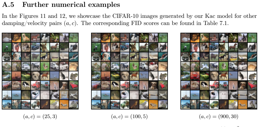
- The mean-reverting Kac process $M_t=f(t)X_0+K_{g(t)}$ with $f(1)=0$ reaches exactly the Kac latent at time $1$, and its conditional velocity has the closed form (7.2), which the CIFAR-10 experiments show can match flow-matching FID scores.
- Because the componentwise decomposition (Lemma 6.1) does not use any Markov property, the same conditional-velocity decomposition applies to any forward process with independent coordinates, as the paper notes in Remark 6.4.
Reading between the lines
- The paper leaves implicit that the closed-form conditional velocity (6.5) can be reused as a fixed teacher for few-step distillation or for likelihood-type evaluation without additional trajectory sampling; the conclusion mentions distillation only as a direction for future work.
- The Kac latent is compactly supported with atoms at $\pm c$ per coordinate in the variance-exploding formulation, so unlike a Gaussian prior it imposes hard spatial limits on generated samples; whether this helps or hurts under distribution shift is not tested in the paper.
- One could also vary the damping and speed per coordinate, which the paper allows in principle but does not exploit; this is a natural design choice for heterogeneous data such as images with different spatial scales.
Editorial analysis
A structured set of objections, weighed in public.
Referee Report
Summary. The paper introduces a generative model based on the Kac (telegrapher) process. It derives an explicit conditional velocity field for a d-dimensional process built from independent 1D Kac components (Theorem 6.2, Eq. (6.5)), proves L2 boundedness of the velocity and Lipschitz continuity of the flow in Wasserstein space (Proposition 5.6), and proves a diffusion limit (Theorems 5.4 and 5.7). It then trains a neural network by conditional flow matching using the analytic velocity and reports CIFAR-10 FID scores together with a 2D Dirac-mode toy comparison.
Significance. If the construction is correct, it is an interesting new member of the flow-matching family: it provides an explicit, componentwise velocity that is globally bounded in L2(µt), unlike diffusion flows, and it retains a diffusion limit. The main theoretical statements are clearly organized, and the appendix gives a rigorous distributional proof of the product decomposition lemma and a corrected proof of Lemma 6.1. The paper also makes its code available. However, the claimed advantage over diffusion is not uniformly supported by the experiments, and the theoretical justification of the reverse-ODE step has a regularity gap that is load-bearing for the generative pipeline.
major comments (3)
- [§2, §6; Eq. (2.4), (6.5), Prop. 5.6] Condition (2.4) is the paper's own sufficient condition for the flow ODE (2.5) to represent the probability flow, but it is never verified for the Kac velocity. Proposition 5.6 proves only the L2 bound (2.3), not the local Lipschitz bound (2.4). The conditional velocity (6.5) is discontinuous at the wavefronts: for fixed t, the interior limit as x_i approaches x_i^0 + ct is ct/(t + 2/a), whereas the assigned boundary value is c, and similarly at x_i^0 - ct. Hence Lip(v_t, B) is infinite on any compact set meeting a wavefront, so (2.4) fails. Proposition A.1(iii) provides only a uniform pointwise bound under bounded data, not a Lipschitz estimate. The manuscript therefore does not justify the reverse-flow step by the cited theorem; a regular-Lagrangian-flow argument or an explicit smoothed-velocity approximation is needed. This also affects the heuristic in §7.2 that "spatial regularity improves" with damping, which is stated without a quantitative statement.
- [Theorem 5.4, Eq. (5.6)] The bound (5.6) cannot hold as stated because it is not homogeneous in f0: replacing f0 by λf0 multiplies the left-hand side by λ while leaving the right-hand side unchanged. The statement must include a norm of f0 on the right-hand side (for example ||f0||_{H^2} or ||f0||_{L^2}) or be restricted to normalized f0. The same omission propagates to Theorem 5.7 and Remark 5.5. As written, the diffusion-limit result is false for arbitrary f0 ∈ H^2(R^d).
- [Abstract, §7, Table 7.1] The abstract's unqualified claim of "advantages over diffusion models" is not uniformly supported by the reported FID numbers. The best Kac score (7.26 for a=900, c=10, g(t)=t^2) is only marginally better than the implemented FM baseline (7.59), and no error bars, multiple seeds, or statistical tests are reported. The diffusion baseline for g(t)=t (FID 82.27) is a known weak configuration. The clear qualitative advantage appears in the 2D Dirac-mode toy experiment (Figure 5). The claim should be qualified to "comparable or better in specific settings" unless the experimental evidence is strengthened.
minor comments (5)
- [Abstract] "Lipschitz continuous in the Wasserstein distance" should be phrased as "Lipschitz continuous as a curve in the Wasserstein space," since Lipschitz continuity is a property of the map t ↦ µ_t.
- [Corollary 6.3 and §7] Corollary 6.3 assumes that X0 has a density f0, while the numerical pipeline uses empirical/atomic data. The relation between the empirical CFM loss and the marginal velocity formula (6.8) should be stated explicitly for the atomic case.
- [Figure 8 and §7.2] The phrase "exploding Lipschitz constants" in the caption of Figure 8 is not quantified. If the derivative of the velocity is indeed unbounded near the wavefronts for small damping, a short asymptotic formula for the relevant coefficient would make the heuristic precise.
- [Appendix A.4, Algorithm 2] The precomputed inverse-CDF table for the continuous part of the Kac density is not described (grid size, interpolation method, and accuracy). Adding these details would improve reproducibility.
- [§3, Eq. (3.1)] In the first example, the calculation of v_t from the coupling should be explicitly identified as the conditional expectation E[y | x_t = x], since the displayed formula is otherwise not immediate.
Circularity Check
No significant circularity: the conditional velocity formula is derived from the Kac distribution with independent existence, and tuned hyperparameters enter only experiments, not the derivation.
full rationale
The central derivation is self-contained. Theorem 4.4 does not define the velocity to be the formula; it assumes existence of any weak-solution velocity field for the Kac distribution and proves that such a field must equal the quotient of the flux J by the density u, with existence supplied independently by Proposition 5.6 via sample-path Lipschitz estimates and the Ambrosio-Gigli-Savare AC^2 theorem. The multivariate decomposition in Lemma 6.1 and Theorem 6.2 is a direct product-rule computation with a rigorous weak-form proof in Appendix A.2, so formula (6.5) is derived rather than fitted. The diffusion-limit results are supported by external classical sources (Kac, Janssen, Griego-Hersh, Nualart), not by the present authors' own prior work. The self-citations that occur, such as [8] and [49], are motivational or secondary restatements of external flow-matching theorems and are not load-bearing for the main results. The skeptical concern about missing Lipschitz regularity for the reverse ODE, condition (2.4), is a genuine correctness or regularity gap but not a circularity: the paper does not assume the conclusion it purports to prove; it simply does not establish the additional regularity needed for ODE well-posedness in full generality. No fitted parameter is renamed as a prediction, and no load-bearing step reduces to its own input by construction.
Assumptions & free parameters
free parameters (3)
- Damping parameter a =
25, 100, 900 in main CIFAR experiments
- Wave speed c =
1, 2, 3, 4, 5, 10, 20, 30
- Time schedule pair (f, g) =
(1-t, t) and (1-t, t^2)
assumptions (5)
- standard math Feynman-Kac representation of the telegrapher equation by the Kac process (Theorem 4.1, Kac [22], Kabanov [21])
- standard math Existence of velocity fields for absolutely continuous Wasserstein curves (Ambrosio-Gigli-Savare Theorem 8.3.1)
- standard math Analytic distribution formula for the Kac process starting at a Dirac point (equation (4.7), attributed to Janssen [20])
- standard math Cosine operator bound for undamped wave solutions (Lutz [29], used in Theorem 5.4)
- domain assumption Bounded data support in the mean-reverting generative setting
Cite this review
Pith. "Pith review of Telegrapher's Generative Model via Kac Flows." pith.science (2026). https://pith.science/paper/LHIT7H6Q
@misc{pith2026250620641,
  author       = {Pith},
  title        = {Pith review of: Telegrapher's Generative Model via Kac Flows},
  year         = {2026},
  howpublished = {\url{https://pith.science/paper/LHIT7H6Q}},
  note         = {Machine review of arXiv:2506.20641}
}
read the original abstract
We break the mold in flow-based generative modeling by proposing a new model based on the damped wave equation, also known as telegrapher's equation. Similar to the diffusion equation and Brownian motion, there is a Feynman-Kac type relation between the telegrapher's equation and the stochastic Kac process in 1D. The Kac flow evolves stepwise linearly in time, so that the probability flow is Lipschitz continuous in the Wasserstein distance and, in contrast to diffusion flows, the norm of the velocity remains globally bounded. Furthermore, the Kac model has the diffusion model as its asymptotic limit. We extend these considerations to a multi-dimensional stochastic process which consists of independent 1D Kac processes in each spatial component. We show that this process gives rise to an absolutely continuous curve in the Wasserstein space and analytically compute the conditional velocity field when starting in a Dirac point. Using the framework of flow matching, we train a neural network to approximate the velocity field and use it for sample generation. Our numerical experiments demonstrate the scalability of our approach, and show its advantages over diffusion models.
Figures


Figures from the paper (11 more)




Forward citations
Cited by 2 Pith papers
-
Provable Diffusion Posterior Sampling for Bayesian Inversion
A diffusion posterior sampler using Monte Carlo Langevin score estimation and warm start is proven to converge in Wasserstein-2 distance under semi-log-concavity and sub-Gaussian assumptions, and outperforms DPS/TV on...
-
Adapting Noise to Data: Generative Flows from 1D Processes
A flow-matching framework that learns each coordinate's latent noise via quantile functions, fitting the noise to the data so transport paths shorten.
Reference graph
Works this paper leans on
-
[1]
M. S. Albergo, N. M. Boffi, and E. Vanden-Eijnden. Stochastic interpolants: A unifying framework for flows and diffusions.arXiv:2303.08797, 2023
arXiv 2023
-
[2]
M. S. Albergo and E. Vanden-Eijnden. Building normalizing flows with stochastic interpolants. ICLR, 2022
work page 2022
-
[3]
L. Ambrosio, E. Brué, and D. Semola.Lectures on Optimal Transport. UNITEXT. Springer Nature, 2021
work page 2021
-
[4]
L. Ambrosio, N. Gigli, and G. Savaré.Gradient Flows. Lectures in Mathematics ETH Zürich. Birkhäuser, Basel, 2nd edition, 2008
work page 2008
-
[5]
D. Blessing, J. Berner, L. Richter, and G. Neumann. Underdamped diffusion bridges with applications to sampling.ICLR, 2025
work page 2025
-
[6]
G. Brunick and S. Shreve. Mimicking an Itô process by a solution of a stochastic differential equation.The Annals of Applied Probability, 23(4):1584––1628, 2013
work page 2013
- [7]
-
[8]
J. Chemseddine, C. Wald, R. Duong, and G. Steidl. Neural sampling from Boltzmann densities: Fisher-Rao curves in the Wasserstein geometry.ICLR, 2025. 25
work page 2025
Show all 53 references
-
[9]
R. T. Q. Chen. torchdiffeq, 2018
2018
-
[10]
Chen and E
Y. Chen and E. Vanden-Eijnden. Scale-adaptive generative flows for multiscale scientific data. arXiv:2509.02971, 2025
2025 arXiv
-
[11]
M. Chester. Second sound in solids.Physical Review, 131:2013–2015, 1963
2013
-
[12]
Dockhorn, A
T. Dockhorn, A. Vahdat, and K. Kreis. Score-based generative modeling with critically-damped Langevin diffusion.ICLR, 2022
2022
-
[13]
S. N. Ethier and T. G. Kurtz.Markov Processes: Characterization and Convergence. Wiley, 1986
1986
-
[14]
Griego and R
R. Griego and R. Hersh. Theory of random evolutions with applications to partial differential equations.Transactions of the American Mathematical Society, 156:405–418, 1971
1971
-
[15]
W. Guo, M. Tao, and Y. Chen. Complexity analysis of normalizing constant estimation: from Jarzynski equality to annealed importance sampling and beyond.arXiv:2502.04575, 2025
2025 arXiv
-
[16]
I. Gyöngy. Mimicking the one-dimensional marginal distributions of processes having an Itô differential.Probabability Theory and Related Fields, 71:501–516, 1986
1986
-
[17]
W. Han, C. Meng, C. D. Manning, and S. Ermon. DistillKac: Few-step image generation via damped wave equations.ICLR, 2026
2026
-
[18]
Holderrieth, M
P. Holderrieth, M. Havasi, J. Yim, N. Shaul, I. Gat, T. Jaakkola, B. Karrer, R. T. Q. Chen, and Y. Lipman. Generator matching: Generative modeling with arbitrary Markov processes. ICLR, 2025
2025
-
[19]
J. Hui, X. Lihu, and Y. Qingshan. Functional large deviations for Kac–Stroock approximation to a class of Gaussian processes with application to small noise diffusions.Journal of Theoretical Probability, 37(4):3015–3054, 2024
2024
-
[20]
A. Janssen. The distance between the Kac process and the Wiener process with applications to generalized telegraph equations.Journal of Theoretical Probability, 3(2):349–360, 1990
1990
-
[21]
Y. M. Kabanov. On the probabilistic representation of a solution of the telegraph equation. Theory of Probability and its Applications, 37:379–380, 1993
1993
-
[22]
M. Kac. A stochastic model related to the telegrapher’s equation.Rocky Mountain Journal of Mathematics, 4(3):497–509, 1974
1974
-
[23]
D. Kim, S. Shin, K. Song, W. Kang, and I.-C. Moon. Soft truncation: A universal training technique of score-based diffusion model for high precision score estimation.ICML, 2022
2022
-
[24]
Lipman, R
Y. Lipman, R. Chen, H. Ben-Hamu, M. Nickel, and M. Le. Flow matching for generative modeling.ICLR, 2023
2023
-
[25]
Lipman, M
Y. Lipman, M. Havasi, P. Holderrieth, N. Shaul, M. Le, B. Karrer, R. T. Q. Chen, D. Lopez-Paz, H. Ben-Hamu, and I. Gat. Flow Matching Guide and Code.arXiv:2412.06264, 2024
2024 arXiv
-
[26]
Q. Liu. Rectified flow: A marginal preserving approach to optimal transport.arXiv:2209.14577, 2022. 26
2022 arXiv
-
[27]
X. Liu, C. Gong, and Q. Liu. Flow straight and fast: Learning to generate and transfer data with rectified flow.ICLR, 2023
2023
-
[28]
Z. Liu, D. Luo, Y. Xu, T. Jaakkola, and M. Tegmark. GenPhys: from physical processes to generative models.arXiv:2304.02637, 2023
2023 arXiv
-
[29]
D. Lutz. Which operators generate cosine operator functions?Atti della Accademia Nazionale dei Lincei. Classe di Scienze Fisiche, Matematiche e Naturali. Rendiconti, Serie 8, 63(5):314–317, 1977
1977
-
[30]
Martin, A
S. Martin, A. Gagneaux, P. Hagemann, and G. Steidl. PnP-Flow: Plug-and-play image restoration with flow matching.ICLR, 2025
2025
-
[31]
Masoliver and G
J. Masoliver and G. H. Weiss. Finite-velocity diffusion.European Journal of Physics, 17:190–196, 1996
1996
-
[32]
Maurais and Y
A. Maurais and Y. Marzouk. Sampling in unit time with kernel Fisher-Rao flow.ICML, 2024
2024
-
[33]
Máté and F
B. Máté and F. Fleuret. Learning interpolations between Boltzmann densities.Transactions on Machine Learning Research, 2023
2023
-
[34]
A. Q. Nichol and P. Dhariwal. Improved denoising diffusion probabilistic models. InInternational conference on machine learning, pages 8162–8171. PMLR, 2021
2021
-
[35]
M. Nualart. Distributional solutions for damped wave equations.Electronic Journal of Differential Equations, 2020(131):1–16, 2020
2020
-
[36]
N. Nüsken. Stein transport for Bayesian inference.arXiv:2409.01464, 2024
2024 arXiv
-
[37]
Obukhov, M
A. Obukhov, M. Seitzer, P.-W. Wu, S. Zhydenko, J. Kyl, and E. Y.-J. Lin. High-fidelity performance metrics for generative models in pytorch, 2020
2020
-
[38]
H. G. Othmer and T. Hillen. The diffusion limit of transport equations derived from velocity- jump processes.SIAM Journal on Applied Mathematics, 61(3):751–775, 2000
2000
-
[39]
Pidstrigach
J. Pidstrigach. Score-based generative models detect manifolds.NeurIPS, 2022
2022
-
[40]
Plonka, D
G. Plonka, D. Potts, G. Steidl, and M. Tasche.Numerical Fourier Analysis. Birkhäuser, Basel, 2nd edition, 2023
2023
-
[41]
Sohl-Dickstein, E
J. Sohl-Dickstein, E. Weiss, N. Maheswaranathan, and S. Ganguli. Deep unsupervised learning using nonequilibrium thermodynamics. In F. Bach and D. Blei, editors,Proceedings of the 32nd International Conference on Machine Learning, volume 37 ofProceedings of Machine Learning Re...
2015
-
[42]
Song and S
Y. Song and S. Ermon. Generative modeling by estimating gradients of the data distribution. NeurIPS, 2019
2019
-
[43]
Y. Song, J. Sohl-Dickstein, D. P. Kingma, A. Kumar, S. Ermon, and B. Poole. Score-based generative modeling through stochastic differential equations.ICLR, 2021
2021
-
[44]
Stroock.Lectures on Topics in Stochastic Differential Equations
D. Stroock.Lectures on Topics in Stochastic Differential Equations. Tata Institute of Funda- mental Research & Springer, 1982. 27
1982
-
[45]
J. Sun, J. Berner, L. Richter, M. Zeinhofer, J. Müller, K. Azizzadenesheli, and A. Anandkumar. Dynamical measure transport and neural PDE solvers for sampling.arXiv:2407.07873, 2024
2024 arXiv
-
[46]
R. C. Tautz and I. Lerche. Application of the three-dimensional telegraph equation to cosmic-ray transport.Research in Astronomy and Astrophysics, 16(10):162–170, 2016
2016
-
[47]
A. Tong, K. Fatras, N. Malkin, G. Huguet, Y. Zhang, J. Rector-Brooks, G. Wolf, and Y. Bengio. Improving and generalizing flow-based generative models with minibatch optimal transport. Transactions on Machine Learning Research, pages 1–34, 2024
2024
-
[48]
Vernotte
P. Vernotte. Les paradoxes de la theorie continue de l’équation de la chaleur.Comptes Rendus., 246:3154–3155, 1958
1958
-
[49]
Wald and G
C. Wald and G. Steidl. Flow Matching: Markov kernels, stochastic processes and transport plans. InVariational and Information Flows in Machine Learning and Optimal Transport, Oberwolfach Seminars. Vol. 56, pages 185–254. Birkhäuser, 2025
2025
-
[50]
Y. Xu, Z. Liu, M. Tegmark, and T. Jaakkola. Poisson flow generative models.NeurIPS, 2022
2022
-
[51]
Zhang, W
B. Zhang, W. Yu, and M. Mascagni. Revisiting Kac’s method: A Monte Carlo algorithm for solving the telegrapher’s equations.Mathematics and Computers in Simulation, 156:176–198, 2018
2018
-
[52]
Y. Zhu, K. Zhang, J. Liang, J. Cao, B. Wen, R. Timofte, and L. Van Gool. Denoising diffusion models for plug-and-play image restoration. InIEEE/CVF Conference on Computer Vision and Pattern Recognition (CVPR) Workshop, pages 1219–1229, 2023. 28 A Appendix: Additional Material ...
2023
-
[53]
Therefore, the choiceg(t) := t isnot admissible for the diffusion case, but valid for the Kac framework
A bound on the norm∥vt∥L2(µt) similar to(A.1) can also be obtained for the stochastic interpolant (7.3), assuming that f and √g are Lipschitz continuous. Therefore, the choiceg(t) := t isnot admissible for the diffusion case, but valid for the Kac framework. Table 7.1 exactly ...
Reviewed August 6, 2026 · model on record in the stance chip above.
Discussion (0). Sign in to comment.