Feature Prediction in Quantum Graph Recurrent Neural Networks with Applications in Information Hiding

Jawaher Kaldari; Saif Al-Kuwari

REVIEW 5 major objections 7 minor 23 references

Feature Prediction in Quantum Graph Recurrent Neural Networks with Applications in Information Hiding

T0 review · 5 major / 7 minor · reviewed 2026-08-06 · deepseek-v4-flash

Challenge this review Re-run · record.json Download PDF Read on arXiv ↗

Pith's one-line read A quantum graph recurrent neural network, trained only on time-evolved states, can reconstruct hidden node features of a classical graph with enough fidelity to preserve near-perfect classification.

desk verdict A clear proof-of-concept for Hamiltonian-parameter recovery on classical data, but the evaluation is cherry-picked and the abstract overstates the results. read the letter →

arxiv 2506.23144 v1 pith:MVET753B submitted 2025-06-29 quant-ph

Jawaher Kaldari , Saif Al-Kuwari This is my paper

classification quant-ph

keywords quantumgraphrecurrentneuralnetworkfeaturereconstructionHamiltonianlearningtransverse-fieldIsingmodelinformationhidingsteganographySWAPtestnodefeatures

verification ladder T0 review T1 audit T2 compute T3 formal

The pith

A machine-rendered reading of the paper's core claim, the machinery that carries it, and where it could break.

The reading

This paper tries to show that a quantum graph recurrent neural network (QGRNN), originally built to learn Hamiltonians of quantum spin systems, can also recover the node features of an ordinary classical graph from nothing but time-evolved quantum states. Features from Iris and PCA-reduced MNIST are embedded as node parameters in a transverse-field Ising Hamiltonian; the QGRNN learns those parameters by matching time-evolved states, and the reconstructed features are close enough that classical classifiers achieve near-perfect accuracy. The same reconstruction mechanism is then turned into an information-hiding scheme, where words are embedded as node values and retrieved only by someone holding the initial and time-evolved states. If this is right, classical graph data can be processed through a quantum Hamiltonian-learning pipeline and then recovered, with direct uses in quantum-enhanced feature extraction and quantum steganography.

What carries the argument

The load-bearing object is the QGRNN ansatz built from the transverse-field Ising Hamiltonian $H(\alpha) = \alpha^{(1)}_{i,j}\sum_{(i,j)}\sigma^z_i\sigma^z_j + \alpha^{(2)}_i\sum_i\sigma^z_i + \sum_i\sigma^x_i$, where $\alpha^{(1)}$ and $\alpha^{(2)}$ are the edge and node weights that carry the embedded classical features. The network approximates the time-evolution unitary $e^{-itH(\alpha)}$ with a Trotter-Suzuki product of Pauli rotations, and training minimizes the average negative fidelity $- \frac{1}{N}\sum_i |\langle\psi(t_i)| U_H(\beta,\delta)|\psi_0\rangle|^2$ between QGRNN-prepared states and the given time-evolved states, with the overlap measured by a SWAP test. The repeated application of the same parameterized layers is what lets a single set of parameters drive the state-matching, and the learned $\beta$ are read out as the predicted node features.

What would settle it

A concrete falsifying test: choose two different node-feature assignments whose time-evolved states are identical at all sampled times under the chosen Hamiltonian, run the QGRNN recovery on each, and check whether the optimization can tell them apart; if such collisions are easy to construct, the reconstruction claim is not generally valid. A simpler version is to run the reported training with all evolution times near zero, where the time-evolved states carry almost no information.

Watch

Extended reading notes

Core claim

On the paper's own terms, the central discovery is that QGRNN, applied to classical datasets encoded as graph Hamiltonians, reconstructs the hidden node features from time-evolved states alone with small error (MSE below about 0.006 on Iris and below about 0.002 on PCA-reduced MNIST, cosine similarity above 0.999), and the reconstructed features preserve class structure well enough that all tested classical classifiers reach 100% accuracy on the reconstructed samples. The paper further claims that the same parameter-recovery process can hide short messages: words mapped to node values are recovered perfectly for 10- and 20-word dictionaries, with degradation at a 40-word dictionary that the authors attribute to tighter numerical spacing rather than to QGRNN reconstruction quality.

Load-bearing premise

The paper assumes that the particular random initial states and sampled evolution times carry enough information to uniquely fix the node parameters that encode the data; if that identifiability fails, the recovered features need not match the original features.

Editorial extensions

If this is right

Classical graph data whose features are embedded in a graph Hamiltonian can be processed without seeing the graph itself: the time-evolved states are the only input QGRNN needs.
The reconstructed Iris and PCA-reduced MNIST features are close enough to the originals that all tested classical classifiers, trained on the original features, classify them perfectly, so feature reconstruction preserves the information needed for downstream tasks.
Message retrieval in the information-hiding scheme is near-perfect for 10- and 20-word dictionaries across sentence lengths, and degrades only at a 40-word dictionary where word values are spaced more tightly.
Larger graphs (six-node MNIST versus four-node Iris) do not degrade reconstruction quality, supporting the paper's scalability claim.

Reading between the lines

Editorial extensions of the paper, not claims the author makes directly.

Going beyond the paper, the near-perfect reconstruction means the scheme's confidentiality is effectively the secrecy of the initial states and evolution times; if those are shared classically, the no-cloning theorem adds little, since the information needed for retrieval is already classical.
A testable extension the paper motivates but does not run: encode data in edges as well as nodes and check whether the same Hamiltonian-parameter recovery doubles the hidden-message capacity per graph size.
The reported results use only six to ten samples per dataset, so a natural scaling test is to increase graph size and sample count while measuring cosine similarity; that curve would show whether reconstruction remains exact outside the proof-of-concept regime.

Share X Bluesky LinkedIn Reddit HN

Editorial analysis

A structured set of objections, weighed in public.

Desk editor's note, referee report, and a circularity audit.

Desk Editor's Note

read the letter

Quick take: the title promises feature prediction in QGRNN for classical data, but what's actually shown is Hamiltonian parameter recovery on six Iris and ten MNIST samples. The method is a straightforward extension of Verdon et al.'s QGRNN: encode features as node weights, evolve, then optimize the ansatz to match the time-evolved states. That part is fine and the convergence plots show it works for these small graphs. The information-hiding application—embedding words as node values and retrieving them by running the same optimization—is a legitimate new use, though it's essentially classical encoding with a quantum dressing.

The problem is the evaluation. Section 4.4 says they trained classifiers on the original data, then only embedded points that were already correctly classified. Tables 7 and 9 are 100% by construction; they tell you nothing about whether the reconstructed features preserve class structure. The feature-prediction tables cover six and ten samples, with no error bars, no repeated seeds, no holdout. That cannot support the abstract's 'scalability and robustness.' The information-hiding results are more honest: Table 10 shows accuracy dropping to 40% for a 40-word dictionary, which the text acknowledges is due to spacing, but the abstract still says 'minor degradation.' That's an overstatement.

The identifiability question is real but secondary. The paper uses random initial states instead of low-energy states, with a footnote justifying it; there's no analysis of whether the time-evolved states uniquely determine the parameters. For these tiny graphs the optimizer seems to find the right values, but without a uniqueness or stability argument the reader can't tell if the method would work on any graph that isn't trivially invertible.

None of this is fatal to the idea. A proof-of-concept with small graphs is fine if it's reported as such. What's not fine is the gap between the abstract and the evidence. The fix is straightforward: run the reconstruction on a proper random subset, report error bars, and either fix the information-hiding claim or drop it from the abstract.

My take: it deserves a serious referee—the QML-for-classical-graphs direction is worth checking—but I would send it back for major revision, and I would not cite it in its current form.

Referee Report

5 major / 7 minor

Summary. The manuscript extends Quantum Graph Recurrent Neural Networks (QGRNNs), originally designed to learn Hamiltonians of quantum systems, to classical graph-structured data. The authors embed classical features (Iris features and PCA-reduced MNIST components) as node parameters of a transverse-field Ising Hamiltonian, simulate time evolution, and then train QGRNN to recover those parameters from the time-evolved states. The recovered features are fed into classical classifiers, and the same reconstruction idea is used to design an information-hiding scheme where words are encoded as node values and retrieved via QGRNN. The paper reports low reconstruction error and near-perfect classification on small samples, and proposes the method as a basis for quantum steganography.

Significance. If the central claim were established, this would be a novel and interesting application of Hamiltonian learning as a feature-reconstruction primitive for classical data, with a possible quantum information-hiding primitive. The idea is clearly stated and testable, and the authors provide per-sample numerical tables rather than only aggregate statistics. However, the evidence as presented is far too weak to support the abstract's claims: the classification evaluation is based on preselected easy samples, the feature-prediction results are point estimates on six and ten hand-picked samples with no error bars, no holdout sets, and no baseline comparisons, and the information-hiding results contradict the abstract's 'minor degradation' statement. No code, simulator version, or reproducibility data is provided. The paper's contribution is therefore currently a proposal rather than a demonstrated result.

major comments (5)

[§4.4.1, §4.4.2, Tables 7 and 9] The classification evaluation does not support the 'near-perfect classification' claim. The authors state that classifiers were trained on the original data and that only data points that were correctly classified were embedded into graphs and then processed by QGRNN. Tables 7 and 9 then report 100% accuracy on those preselected points. This protocol selects the easiest cases and cannot distinguish faithful reconstruction from memorization or from the classifier's prior performance on easy samples. The authors should test on a random holdout set that includes both correctly and incorrectly classified original points, and report per-class and cross-validated accuracy with confidence intervals.
[§4.3, Tables 2–5] The feature-reconstruction metrics are computed on only six Iris samples and ten MNIST samples, which are the same preselected, correctly classified points used later in §4.4. These are not random or representative subsets, and there are no repeated seeds, no error bars, and no sensitivity analysis over the free hyperparameters listed in Table 1 (learning rate, Trotter step, tmax, PCA dimension, feature scaling). The reported MSE/RMSE/MAE and cosine-similarity values are point estimates on a tiny, cherry-picked sample and cannot support the general claim of high reconstruction accuracy or scalability.
[§3.3, footnote 1, §4.1] The training protocol is a per-sample consistency check rather than a test of predictive capability. For each sample, the time-evolved states are generated from a Hamiltonian whose node parameters are exactly the features to be recovered, and the cost plots in Figures 3 and 5 show separate optimizations per sample. The replacement of low-energy initial states with randomly initialized states, noted in the footnote in §4.1, is not accompanied by any identifiability or uniqueness analysis; nothing shows that the chosen random initial states and time samples uniquely determine the node parameters. The authors should demonstrate generalization by withholding time points or samples, by using multiple random initial states, and by comparing against a baseline such as direct curve-fitting or a classical inversion method.
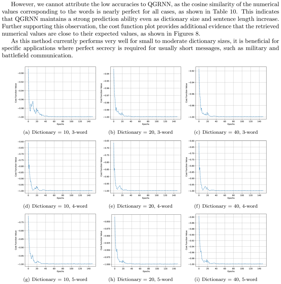
[§5, Table 10] The abstract's claim of 'minor degradation as complexity increases' is directly contradicted by Table 10: for the 40-word dictionary, retrieval accuracy drops to 66.67%, 50%, and 40% for sentences of length 3, 4, and 5, respectively. Additionally, the paper reports cosine similarity of 0.999 in all cases even when accuracy is 40%, which shows that the cosine metric is insensitive to the threshold-level errors that determine retrieval success. The discussion in §5 saying that the low accuracy cannot be attributed to QGRNN is not convincing; if the reconstructed numerical values are that close, the authors need to analyze the error distribution and the decision threshold rather than relying on cosine similarity.
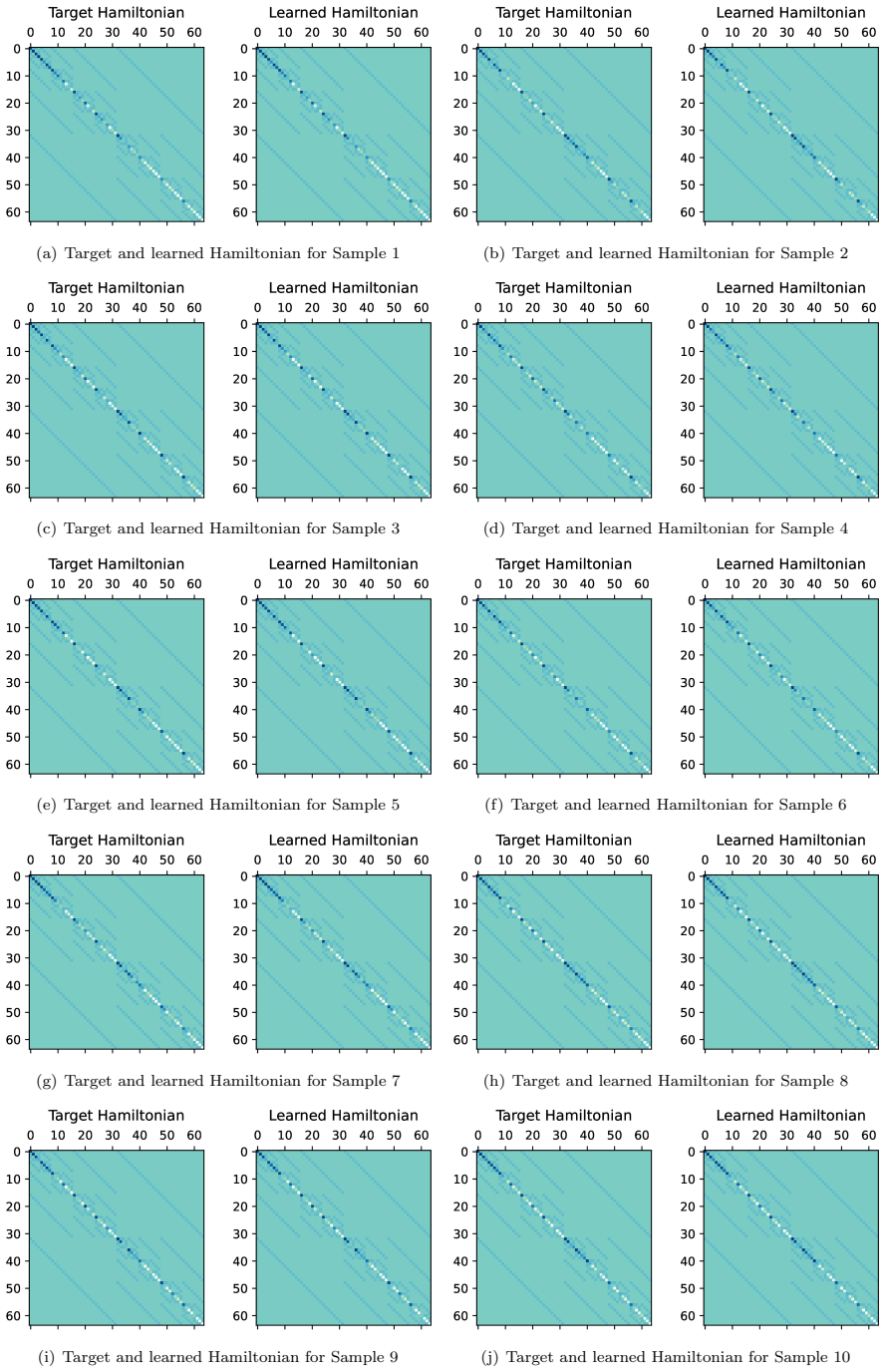
[§3.2, §4.3.1, Figures 4 and 6] The Hamiltonian comparison used as a validation metric is weak and potentially misleading. In §4.3.1 the authors themselves state that 'the Hamiltonian itself is not strictly related in our classical graph setting,' yet Figures 4 and 6 are presented as evidence that QGRNN 'captures the underlying relationships in the graph structure.' Furthermore, edges are said to be randomly initialized and not used for data embedding, so the edge terms in the learned Hamiltonian have no clear target. The authors should either remove this validation argument or clearly define what graph structure the Hamiltonian is supposed to recover.

minor comments (7)

[§2.1] There is a typo: 'molcules' should be 'molecules.'
[§2.3] The text uses 'anzats' where 'ansatz' is intended.
[§4.2] The MSE formula has a typo: 'wher yi' should be 'where yi.'
[§3.2 and §4.3] Please clarify whether the edge parameters α(1) in Eq. (3) are optimized, fixed at random values, or treated as known; the Hamiltonian comparison figures include edge structure, but the data embedding uses only node features.
[§4.1, footnote 1] The authors state that randomly initialized quantum states are 'precomputed and reused'; it should be stated explicitly whether the same initial states are used for all samples and for the training and evaluation phases, since this affects the conclusions about generalization.
[§5] There is a typo in the first paragraph: 'the use of QRNN' should read 'the use of QGRNN.'
[General] The manuscript contains no code, no simulation software version, no random seed specification, and no data availability statement; this limits reproducibility and should be addressed if the paper is revised.

Circularity Check

2 steps flagged · score 6.0 of 10

Feature 'prediction' is an in-sample parameter fit: β is optimized against time-evolved states generated by H_target(θ), so β→θ measures training fit; the 100% classification tables are additionally preselected from already-correctly-classified points.

fitted input called prediction [Section 2.3.1 (Eqs. 9-10), applied in Section 3.3 and evaluated in Section 4.3]
"|ψt⟩ ≡U (t) |ψ0⟩ = e−itHtarget (θ) ... Htarget(θ) = θi,j (1) Σ σz i σz j + θi (2) Σ σz i + Σ σx i ... Then the parameters β = {β1, β2} are optimized to increase the similarity between the time-evolved states and the states prepared using the QGRNN: UH (δ, β) |ψ0⟩ ≈ |ψt⟩ As the states converge, β → θ"

The 'actual features' reported in Tables 2 and 4 are the Hamiltonian parameters θ of Eq. (10), and the time-evolved states used for training are generated by exactly those parameters via Eq. (9): |ψ_t⟩ = e^{-itH_target(θ)}|ψ0⟩. The 'predicted features' are the optimized variational parameters β, chosen by minimizing L(β,δ) = -1/N Σ |⟨ψ(t_i)|U_H(β,δ)|ψ0⟩|^2 against those same states. Thus β is fitted to data produced by θ, and reporting MSE/RMSE/MAE/cosine between β and θ measures training-set fit, not predictive accuracy. No held-out samples, seeds, or identifiability analysis separate the optimizer's fit from a genuine prediction; the high accuracy is forced by the optimization objective whenever the ansatz can represent the target Hamiltonian.
other [Section 4.4.1 and Section 4.4.2 (Tables 7 and 9)]
"After training, we selected data points that were correctly classified and embedded them into a graph. We then applied our QGRNN-based methodology to reconstruct the feature values and classified these predicted features using the previously trained models."

The 100% classification results in Tables 7 and 9 are obtained on a subset chosen by the outcome being measured: only points the previously trained classifiers already labeled correctly on the original features were embedded and re-tested. With reconstructed features close to the originals, re-classifying these preselected easy points cannot fail, so the reported accuracy is an artifact of the selection rule. This is selection-on-outcome rather than a test of whether QGRNN's reconstructions preserve class information; it cannot support the abstract's 'near-perfect classification' claim.

full rationale

The central demonstration is a Hamiltonian-parameter recovery simulation: the node features are placed in H_target(θ), time-evolved states are generated from H_target(θ), and the QGRNN variational parameters β are optimized to reproduce those states. Reporting β as a 'prediction' of θ and measuring agreement with θ is therefore a check of the optimizer and of identifiability, not a prediction on unseen data; the paper supplies no identifiability analysis (the footnote in Sec. 4.1 even replaces low-energy states by random states 'since we simulate classical graphs and have full knowledge of the system'). The classification claim is further weakened by the explicit selection of correctly classified data points before embedding, making Tables 7 and 9 tautological. The information-hiding section inherits the same retrieval pipeline and therefore the same in-sample character. There is no self-citation chain: refs [7] and [14] are not by the present authors, and the ansatz is adopted from prior work as normal background. Overall, the central quantitative claims reduce by construction to fitting and selection, giving partial circularity.

Assumptions & free parameters 5 free parameters · 6 assumptions · 0 invented entities

The method has no invented physical entities. It relies on a number of domain assumptions: the Ising ansatz for data encoding, the sufficiency of time-evolved states for parameter recovery, the substitution of random for low-energy initial states, and the Trotter approximation. The feature scaling, PCA dimension, Trotter step size, and evolution time are hand-chosen and affect the reported accuracies.

free parameters (5)

Feature scaling range = [0, 5]
Features are scaled to [0,5] to improve training stability (Section 3.1). This changes the Hamiltonian parameter scale and affects reconstruction accuracy.
Number of PCA components = 6
MNIST images are reduced to six principal components to fit the qubit budget (Section 3.1). This arbitrary choice affects the information content and graph size.
Trotter step size = 0.01
Set in Table 1; controls the Trotter approximation error in the QGRNN ansatz and thus the fidelity of the learned evolution.
Maximum evolution time = 0.5
Set in Table 1; determines the set of time-evolved states used as training data.
Dictionary value range = [-4, 5]
Chosen for the word-to-number mapping in the information hiding experiments (Section 5); affects the spacing between encoded words and retrieval difficulty.

assumptions (6)

domain assumption The transverse-field Ising model Hamiltonian (Eq. 3) is an appropriate ansatz for encoding classical graph features.
Adopted from QGRNN literature; assumes feature values can be represented as node and edge weights in H(alpha).
domain assumption Time-evolved states generated from the target Hamiltonian contain sufficient information to recover the node parameters.
Central identifiability assumption; not proven. The set of initial states and evolution times may not uniquely determine theta.
ad hoc to paper Randomly initialized states can substitute for low-energy states in QGRNN training.
Footnote 1 in Section 4.1 explicitly deviates from the original QGRNN protocol, which assumes access to low-energy states prepared by VQE.
domain assumption The Trotter-Suzuki decomposition with delta=0.01 approximates the time evolution accurately enough for parameter recovery.
Standard approximation, but the error is not bounded in the paper; the chosen delta and t_max affect the fidelity.
standard math The SWAP test provides an accurate estimate of fidelity in the simulation.
Standard quantum information result, but the simulation details are not provided.
domain assumption The identity of the sigma_x term coefficient (set to 1) in Eq. 3 is known and fixed.
The target Hamiltonian has a known transverse field coefficient; in real systems this may be unknown, making the parameter recovery easier than the claimed scenario.

how reviews work

0 comments

Cite this review

Pith. "Pith review of Feature Prediction in Quantum Graph Recurrent Neural Networks with Applications in Information Hiding." pith.science (2026). https://pith.science/paper/MVET753B

@misc{pith2026250623144,
  author       = {Pith},
  title        = {Pith review of: Feature Prediction in Quantum Graph Recurrent Neural Networks with Applications in Information Hiding},
  year         = {2026},
  howpublished = {\url{https://pith.science/paper/MVET753B}},
  note         = {Machine review of arXiv:2506.23144}
}

read the original abstract

Graphs are a fundamental representation of complex, nonlinear structured data across various domains, including social networks and quantum systems. Quantum Graph Recurrent Neural Networks (QGRNNs) have been proposed to model quantum dynamics in graph-based quantum systems, but their applicability to classical data remains an open problem. In this paper, we leverage QGRNNs to process classical graph-structured data. In particular, we demonstrate how QGRNN can reconstruct node features in classical datasets. Our results show that QGRNN achieves high feature reconstruction accuracy, leading to near-perfect classification. Furthermore, we propose an information hiding technique based on our QGRNN, where messages are embedded into a graph, then retrieved under certain conditions. We assess retrieval accuracy for different dictionary sizes and message lengths, showing that QGRNN maintains high retrieval accuracy, with minor degradation as complexity increases. These findings demonstrate the scalability and robustness of QGRNNs for both classical data processing and secure information hiding, paving the way for quantum-enhanced feature extraction, privacy-preserving computations, and quantum steganography.

Figures

Figures reproduced from arXiv: 2506.23144 by the authors.

**Figure 2.** SWAP test circuit where N is the number of quantum states processed, or the batch size. 3 Methodology Our proposal leverages QGRNN to predict and reconstruct hidden features of a dataset represented as a classical graph, relying solely on time-evolved states when direct access to the graph is unavailable. The reconstructed features are then used as input for classical machine learning models to perform classificatio… view at source ↗

**Figure 3.** Cost function value for all tested Iris samples [PITH_FULL_IMAGE:figures/full_fig_p008_3.png] view at source ↗

Figures from the paper (5 more)

**Figure 4.** Figure 4: A visual representation of the Hamiltonian for all tested Iris samples [PITH_FULL_IMAGE:figures/full_fig_p009_4.png]

**Figure 5.** Figure 5: Cost function value for all tested MNIST samples [PITH_FULL_IMAGE:figures/full_fig_p011_5.png]

**Figure 6.** Figure 6: A visual representation of the Hamiltonian for all tested MNIST samples [PITH_FULL_IMAGE:figures/full_fig_p012_6.png]

**Figure 7.** Figure 7: Accuracy Across Different Dictionary Sizes and Sentence Lengths [PITH_FULL_IMAGE:figures/full_fig_p015_7.png]

**Figure 8.** Figure 8: Cost function value for all dictionary sizes and sentence lengths [PITH_FULL_IMAGE:figures/full_fig_p016_8.png]

Discussion (0). Sign in to comment.

Reference graph

Works this paper leans on

23 extracted references · 17 canonical work pages

[1]

Counterfactual learning on graphs: A survey,

Z. Guo, Z. Wu, T. Xiao, C. Aggarwal, H. Liu, and S. Wang, “Counterfactual learning on graphs: A survey,” Machine Intelligence Research, vol. 22, no. 1, pp. 17–59, 2025

work page 2025
[2]

Graph neural networks for intelli- gent transportation systems: A survey,

S. Rahmani, A. Baghbani, N. Bouguila, and Z. Patterson, “Graph neural networks for intelli- gent transportation systems: A survey,” IEEE Transactions on Intelligent Transportation Systems, vol. 24, no. 8, pp. 8846–8885, 2023

work page 2023
[3]

Graph neural networks in recommender systems: a survey,

S. Wu, F. Sun, W. Zhang, X. Xie, and B. Cui, “Graph neural networks in recommender systems: a survey,” ACM Computing Surveys, vol. 55, no. 5, pp. 1–37, 2022

2022
[4]

A comprehensive survey on graph neural networks,

Z. Wu, S. Pan, F. Chen, G. Long, C. Zhang, and S. Y. Philip, “A comprehensive survey on graph neural networks,” IEEE transactions on neural networks and learning systems, vol. 32, no. 1, pp. 4–24, 2020

work page 2020
[5]

Spatial gating strategies for graph recurrent neural networks,

L. Ruiz, F. Gama, and A. Ribeiro, “Spatial gating strategies for graph recurrent neural networks,” in ICASSP 2020 - 2020 IEEE International Conference on Acoustics, Speech and Signal Processing (ICASSP), 2020, pp. 5550–5554. 17

work page 2020
[6]

Stationary signal processing on graphs,

N. Perraudin and P. Vandergheynst, “Stationary signal processing on graphs,” IEEE Transactions on Signal Processing, vol. 65, no. 13, pp. 3462–3477, 2017

work page 2017
[7]

Quantum graph neural networks,

G. Verdon, T. McCourt, E. Luzhnica, V. Singh, S. Leichenauer, and J. Hidary, “Quantum graph neural networks,” arXiv preprint arXiv:1909.12264, 2019

arXiv 1909
[8]

Quantum machine learning of graph- structured data,

K. Beer, M. Khosla, J. K¨ ohler, T. J. Osborne, and T. Zhao, “Quantum machine learning of graph- structured data,” Physical Review A, vol. 108, no. 1, p. 012410, 2023

work page 2023

Show all 23 references

[9]

Quantum kernels for unattributed graphs using discrete-time quantum walks,

L. Bai, L. Rossi, L. Cui, Z. Zhang, P. Ren, X. Bai, and E. Hancock, “Quantum kernels for unattributed graphs using discrete-time quantum walks,” Pattern Recognition Letters, vol. 87, pp. 96–103, 2017

2017
[10]

Quantum computing in the nisq era and beyond,

J. Preskill, “Quantum computing in the nisq era and beyond,” Quantum, vol. 2, p. 79, 2018

2018
[11]

The ising model: teaching an old problem new tricks,

Z. Bian, F. Chudak, W. G. Macready, and G. Rose, “The ising model: teaching an old problem new tricks,” D-wave systems, vol. 2, pp. 1–32, 2010

2010
[12]

History of the lenz-ising model,

S. G. Brush, “History of the lenz-ising model,” Reviews of modern physics, vol. 39, no. 4, p. 883, 1967

1967
[13]

An introduction to the ising model,

B. A. Cipra, “An introduction to the ising model,” The American Mathematical Monthly, vol. 94, no. 10, pp. 937–959, 1987

1987
[14]

A tutorial on quantum graph recurrent neural network (qgrnn),

J. Choi, S. Oh, and J. Kim, “A tutorial on quantum graph recurrent neural network (qgrnn),” in 2021 International Conference on Information Networking (ICOIN). IEEE, 2021, pp. 46–49

2021
[15]

Quantum phase transitions in transverse field spin models: from statistical physics to quantum information,

A. Dutta, G. Aeppli, B. K. Chakrabarti, U. Divakaran, T. F. Rosenbaum, and D. Sen, “Quantum phase transitions in transverse field spin models: from statistical physics to quantum information,” arXiv preprint arXiv:1012.0653, 2010

2010 arXiv
[16]

Tensorflow quantum: A software framework for quantum machine learning,

M. Broughton, G. Verdon, T. McCourt, A. J. Martinez, J. H. Yoo, S. V. Isakov, P. Massey, R. Halavati, M. Y. Niu, A. Zlokapa et al., “Tensorflow quantum: A software framework for quantum machine learning,” arXiv preprint arXiv:2003.02989, 2020

2003 arXiv
[17]

Optimising trotter- suzuki decompositions for quantum simulation using evolutionary strategies,

B. D. Jones, D. R. White, G. O. O’Brien, J. A. Clark, and E. T. Campbell, “Optimising trotter- suzuki decompositions for quantum simulation using evolutionary strategies,” in Proceedings of the Genetic and Evolutionary Computation Conference, 2019, pp. 1223–1231

2019
[18]

Intro to qaoa,

J. Ceroni, “Intro to qaoa,” Nov 2020. [Online]. Available: https://pennylane.ai/qml/demos/ tutorial qaoa intro/

2020
[19]

Beyond the swap test: optimal estimation of quantum state overlap,

M. Fanizza, M. Rosati, M. Skotiniotis, J. Calsamiglia, and V. Giovannetti, “Beyond the swap test: optimal estimation of quantum state overlap,” Physical review letters, vol. 124, no. 6, p. 060503, 2020

2020
[20]

Swap test-based characterization of quantum processes in universal quantum computers,

P. Ripper, G. Amaral, and G. Tempor˜ ao, “Swap test-based characterization of quantum processes in universal quantum computers,” arXiv preprint arXiv:2208.02893, 2022

2022 arXiv
[21]

The use of multiple measurements in taxonomic problems,

R. A. Fisher, “The use of multiple measurements in taxonomic problems,” Annals of eugenics, vol. 7, no. 2, pp. 179–188, 1936

1936
[22]

Gradient-based learning applied to document recognition,

Y. LeCun, L. Bottou, Y. Bengio, and P. Haffner, “Gradient-based learning applied to document recognition,” Proceedings of the IEEE, vol. 86, no. 11, pp. 2278–2324, 2002

2002
[23]

Perspective chapter: Quantum steganography–encoding secrets in the quantum domain,

A. Agrawal, R. Soni, and A. Tomar, “Perspective chapter: Quantum steganography–encoding secrets in the quantum domain,” 2024. 18

2024

Pith tools

Reviewed August 6, 2026 · model on record in the stance chip above.

[1] [1]

Counterfactual learning on graphs: A survey,

Z. Guo, Z. Wu, T. Xiao, C. Aggarwal, H. Liu, and S. Wang, “Counterfactual learning on graphs: A survey,” Machine Intelligence Research, vol. 22, no. 1, pp. 17–59, 2025

work page 2025

[2] [2]

Graph neural networks for intelli- gent transportation systems: A survey,

S. Rahmani, A. Baghbani, N. Bouguila, and Z. Patterson, “Graph neural networks for intelli- gent transportation systems: A survey,” IEEE Transactions on Intelligent Transportation Systems, vol. 24, no. 8, pp. 8846–8885, 2023

work page 2023

[3] [3]

Graph neural networks in recommender systems: a survey,

S. Wu, F. Sun, W. Zhang, X. Xie, and B. Cui, “Graph neural networks in recommender systems: a survey,” ACM Computing Surveys, vol. 55, no. 5, pp. 1–37, 2022

2022

[4] [4]

A comprehensive survey on graph neural networks,

Z. Wu, S. Pan, F. Chen, G. Long, C. Zhang, and S. Y. Philip, “A comprehensive survey on graph neural networks,” IEEE transactions on neural networks and learning systems, vol. 32, no. 1, pp. 4–24, 2020

work page 2020

[5] [5]

Spatial gating strategies for graph recurrent neural networks,

L. Ruiz, F. Gama, and A. Ribeiro, “Spatial gating strategies for graph recurrent neural networks,” in ICASSP 2020 - 2020 IEEE International Conference on Acoustics, Speech and Signal Processing (ICASSP), 2020, pp. 5550–5554. 17

work page 2020

[6] [6]

Stationary signal processing on graphs,

N. Perraudin and P. Vandergheynst, “Stationary signal processing on graphs,” IEEE Transactions on Signal Processing, vol. 65, no. 13, pp. 3462–3477, 2017

work page 2017

[7] [7]

Quantum graph neural networks,

G. Verdon, T. McCourt, E. Luzhnica, V. Singh, S. Leichenauer, and J. Hidary, “Quantum graph neural networks,” arXiv preprint arXiv:1909.12264, 2019

arXiv 1909

[8] [8]

Quantum machine learning of graph- structured data,

K. Beer, M. Khosla, J. K¨ ohler, T. J. Osborne, and T. Zhao, “Quantum machine learning of graph- structured data,” Physical Review A, vol. 108, no. 1, p. 012410, 2023

work page 2023