One-loop analysis of dark matter constraints in a complex scalar extension of the Standard Model

Chikako Idegawa; Koichi Funakubo

REVIEW 3 major objections 4 minor 39 references

One-loop analysis of dark matter constraints in a complex scalar extension of the Standard Model

T0 review · 3 major / 4 minor · reviewed 2026-08-06 · deepseek-v4-flash

Challenge this review Re-run · record.json Download PDF Read on arXiv ↗

Pith's one-line read This paper argues that one-loop quantum corrections substantially change the dark matter constraints on the complex singlet extension of the Standard Model, shrinking the allowed parameter region and drastically reducing it when the two…

desk verdict A real one-loop calculation in the CxSM, but the headline result about the degenerate-region collapse rests on an acknowledged h1-loop truncation that could break the very cancellation it reports. read the letter →

arxiv 2506.23199 v2 pith:OAVUIXRY submitted 2025-06-29 hep-ph

Koichi Funakubo , Chikako Idegawa This is my paper · ORCID

classification hep-ph

keywords complexsingletextensionscalardarkmatterone-loopeffectivepotentialdirectdetectionconstraintsrelicabundancedegeneratescenariofinitecountertermsannihilation

verification ladder T0 review T1 audit T2 compute T3 formal

The pith

A machine-rendered reading of the paper's core claim, the machinery that carries it, and where it could break.

The reading

The paper argues that quantum corrections at one loop materially change the dark matter phenomenology of the complex singlet extension of the Standard Model, a minimal WIMP (weakly interacting massive particle) model in which the imaginary part of a complex scalar singlet is the dark matter particle. The authors compute the one-loop effective potential, fix the finite counterterms so that the vacuum and mass conditions keep their tree-level form, and feed the one-loop corrected scalar self-interactions into both the dark matter–nucleon scattering amplitude and the annihilation cross section that sets the relic abundance. Their central result is that the allowed parameter region shifts visibly away from the tree-level prediction, and for the nearly degenerate case $m_{h_2}=126$ GeV the region consistent with the LUX-ZEPLIN direct-detection bound and the observed relic density is drastically reduced. If correct, this means tree-level-only scans of this model are not reliable once the couplings involving the dark matter particle are large enough to matter.

What carries the argument

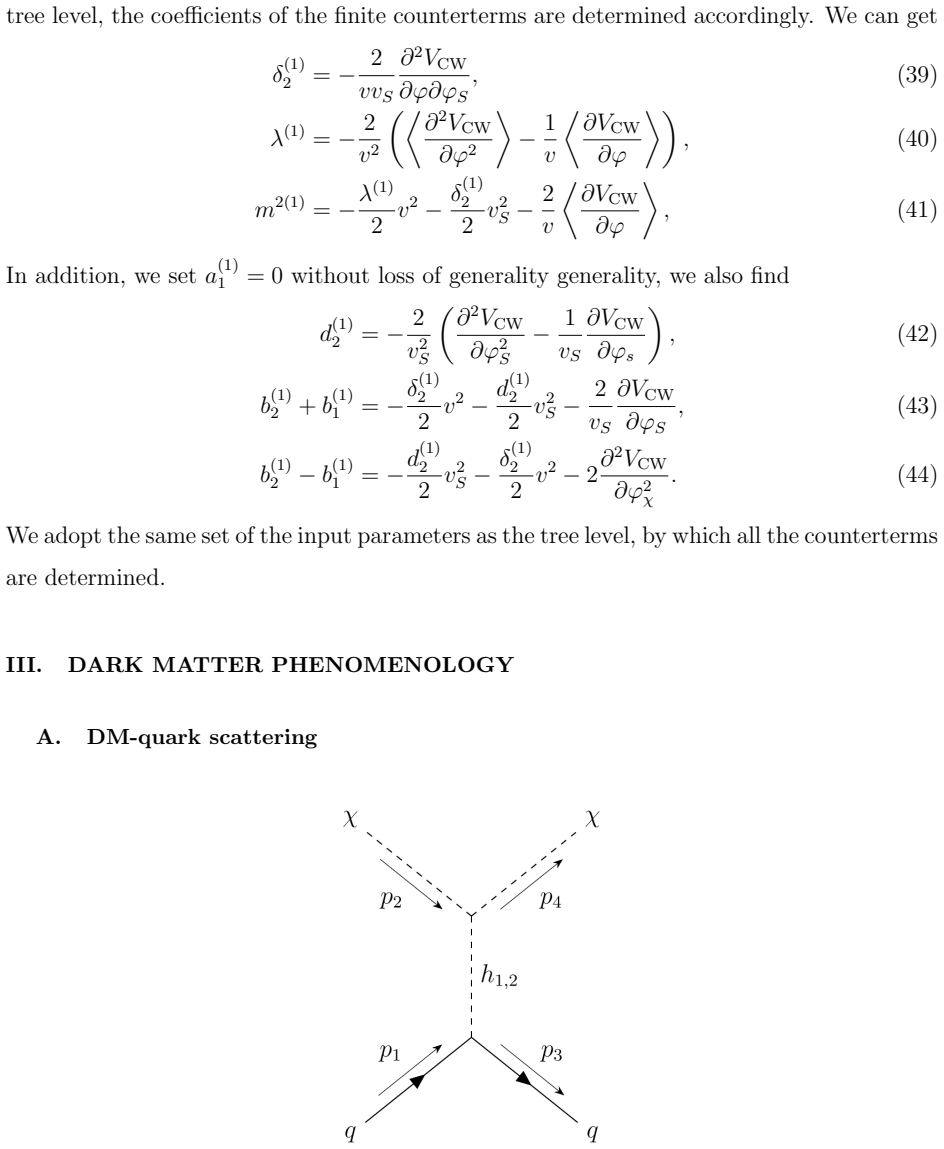
The central object is the complex singlet extension (CxSM) potential with a complex singlet $S$ whose imaginary component $\chi$ is protected by a $\mathbb{Z}_2$ sign-flip symmetry and serves as the dark matter candidate, while the real component mixes with the Higgs doublet through a mixing angle $\alpha$ into mass eigenstates $h_1$ (the 125 GeV Higgs) and $h_2$. The machinery that carries the argument is the one-loop effective potential with the Coleman--Weinberg corrections plus finite counterterms selected so that the tadpole and mass conditions keep their tree-level form; the one-loop corrected vertices $\Gamma_{\chi\chi h_i}$ and $\Gamma_{\chi\chi h_i h_j}$ then enter both the $\chi$-quark scattering amplitude and all dark matter annihilation channels. The loop functions $\varphi_2$ and $\varphi_3$ encode the momentum-dependent corrections, and the counterterms $\delta_2^{(1)}$, $d_2^{(1)}$, $D_1^{(1)}$, $D_2^{(1)}$ absorb the radiative shifts of the couplings. The decisive mechanism is that these radiative shifts move the effective $\chi\chi h_i$ couplings away from the tree-level relation that made the near-degenerate $h_1/h_2$ contributions cancel.

What would settle it

A concrete check would be to recompute the one-loop $\chi$-quark and $\chi\chi$ annihilation amplitudes including the $h_1$-propagator contributions that the paper omits, or to use a renormalization-group-improved effective potential that avoids the negative-mass-squared region, and to compare the resulting LZ-allowed and relic-allowed regions at $m_{h_2}=126$ GeV with the paper's one-loop result. If the $h_1$-loop terms restore the near-degeneracy cancellation for representative benchmark points, the claimed drastic reduction would not survive the full calculation.

Watch

Extended reading notes

Core claim

On the paper's own terms, the discovery is that including the one-loop corrections to the effective potential, the counterterms, and the scalar self-interaction vertices involving the dark matter candidate $\chi$ changes which points in the $(m_{\chi}, v_S, a_1)$ parameter space survive the two main dark matter constraints. At tree level the degenerate scalar scenario, where the two CP-even Higgs mass eigenstates $h_1$ and $h_2$ are nearly equal in mass, cancels the $\chi$-quark scattering amplitude and produces the largest allowed region for $m_{h_2}=126$ GeV. In the one-loop analysis, the radiative corrections to the effective $\chi\chi h_i$ and $\chi\chi h_i h_j$ vertices spoil that cancellation, so the direct-detection cross section is no longer suppressed and the $m_{h_2}=126$ GeV region shrinks drastically. For heavier $m_{h_2}$ the same radiative effects strengthen the effective couplings, making the LZ bound more restrictive while enhancing the annihilation cross section that determines the relic abundance; after all constraints, the one-loop allowed region is generally smaller, and in the near-degenerate case drastically so.

Load-bearing premise

The load-bearing premise is that all one-loop diagrams containing the Standard-Model-like Higgs boson $h_1$ can be left out without changing the answer, because that particle's field-dependent mass squared is negative in part of the field space; if those omitted diagrams are not small, the reported one-loop shifts, especially the drastic shrinking of the $m_{h_2}=126$ GeV region, could be an artifact of the truncation.

Editorial extensions

If this is right

Tree-level-only analyses of the CxSM are insufficient: the one-loop corrected vertices alter both the direct-detection cross section and the relic abundance, so allowed regions computed at tree level can change size or vanish.
For $m_{h_2}=126$ GeV, the degenerate scalar scenario's built-in cancellation is mostly undone by radiative vertex corrections, so the parameter region surviving both the LZ bound and the relic constraint is drastically smaller than the tree-level region.
For heavier $h_2$, the one-loop corrections enhance the effective couplings: the LZ bound excludes more points, while the larger annihilation cross section makes the relic abundance easier to match (or pushes the relic abundance below the observed value for $m_{h_2}=2000$ GeV).
Because the one-loop analysis leaves little room, the paper points to adding scalar cubic couplings $c_1, c_2, c_3$ as a way to free $b_2-b_1$ and the effective $\chi\chi h_i$ vertices and recover viable regions, and it notes that this extension could also help a strong first-order electroweak phase transition.

Reading between the lines

Editorial extensions of the paper, not claims the author makes directly.

An implication the authors do not develop is that the same one-loop vertex corrections should also change indirect-detection signals and collider probes such as invisible Higgs decays or di-Higgs production, so a complete comparison with experiment would extend beyond direct detection and relic abundance.
Because the $h_1$-loop omission is tied to a negative field-dependent mass squared, a natural test is whether a full two-loop or resummed calculation reverses the sign of the one-loop shift; the paper's conclusion that the allowed region shrinks is only as strong as that truncation.
The near-degeneracy cancellation at $m_{h_2}=126$ GeV is a tree-level fine-tuning that radiative corrections partially spoil; one could quantify how large the mass splitting must be for the one-loop allowed region to reappear, which would tell LHC searches how much degeneracy remains phenomenologically viable.
The paper's vacuum-stability check that the $\varphi_{\chi}=0$ vacuum is the global minimum is performed at tree level; extending that check to the one-loop effective potential could rule out or rescue some of the surviving points, especially in the $m_{h_2}=126$ GeV region where stationary points with $\varphi_{\chi}\neq 0$ appear.

Share X Bluesky LinkedIn Reddit HN

Editorial analysis

A structured set of objections, weighed in public.

Desk editor's note, referee report, and a circularity audit.

Desk Editor's Note

read the letter

Short version: the paper computes one-loop corrected DM constraints in the CxSM with explicit counterterms; that is new for this model and the vertex functions are spelled out in detail. The qualitative claim that one-loop corrections weaken the degenerate scalar cancellation is plausible. But the central quantitative result—that the mh2=126 GeV region is 'drastically reduced'—is not supported, because every diagram containing the h1 propagator is omitted, and that is exactly the partner in the tree-level cancellation.

What is genuinely there: the counterterm scheme fixes tadpoles and masses at their tree-level values, which is standard and self-consistent; the expressions for the χχhi vertices at one loop are explicit and not just quoted from a code; and the observation that D1 and D2 get asymmetrical shifts, so the degenerate cancellation (Eq. (50)) becomes imperfect at one loop, is a real point worth taking seriously.

The soft spots, in order of size. First, the h1-loop omission. Appendix A says it is because the field-dependent h1 mass squared is negative somewhere in the (φ,φS) plane; Appendix C repeats it. That reason does not apply at the vacuum, where m_h1^2 > 0, so the loop is well defined there. The omitted diagrams are the same order as the h2 and χ loops actually kept. Because the tree-level degeneracy suppression is a cancellation between h1 and h2 amplitudes, dropping h1 loops asymmetrically changes the two couplings and can create or break the cancellation. The paper gives no estimate of the omitted size, so the 'drastically reduced' claim for mh2=126 GeV is unsupported. The abstract's phrase 'fully included' is simply wrong relative to the body of the paper.

Second, the vertices are evaluated at zero incoming momentum even for s-channel annihilation near the resonance. That is a rough approximation, perhaps acceptable for a first pass, but not the full one-loop treatment the abstract implies.

Third, g*=heff=80 constant is a coarse choice; for low mχ the freeze-out temperature is low enough that g* should vary. Probably a minor issue relative to the above.

Bottom line: worth a serious referee because it is a legitimate first step and the formulas are reproducible in principle, but the referee must push for either the h1-loop contributions or a credible estimate of their size before the central conclusion is accepted. I would not rely on the quantitative plots as they stand. Desk rejection would be wrong; this needs refereeing, not burial.

Referee Report

3 major / 4 minor

Summary. This paper studies the complex singlet extension of the Standard Model (CxSM) with a complex scalar dark matter candidate χ, computing one-loop corrections to the effective potential, the associated finite counterterms, and the scalar self-interactions relevant for direct detection and annihilation. The authors impose LZ direct detection bounds and the observed relic density and compare the resulting allowed parameter regions with the tree-level analysis. Their central claim is that one-loop corrections materially change the phenomenology, in particular that the degenerate scalar scenario at mh2 = 126 GeV, which is viable at tree level, has its allowed region 'drastically reduced' after including one-loop effects (Sec. IV). The paper provides explicit counterterm formulas (39)–(44), closed-form one-loop vertex functions (C25)–(C29), and a parameter scan over mχ, vS, and a1.

Significance. If the one-loop treatment were complete, this paper would provide a useful demonstration that tree-level-only analyses of the CxSM can be misleading, and it would update the status of the degenerate scalar scenario under current LZ and Planck data. The explicit derivation of counterterms and the careful treatment of vacuum stability are assets, and the paper is clearly written in its technical parts. However, the central quantitative claims rest on a truncation that the paper itself acknowledges, and the relic density calculation uses approximations that are too crude for the claimed precision. The paper is therefore a useful starting point, but its main conclusions require additional work before they can be accepted as definitive.

major comments (3)

[Appendix A; Appendix C; Sec. IV] The one-loop calculations omit all diagrams containing an h1 propagator. Appendix A states that h1-loop contributions are omitted because the field-dependent mass squared of h1 is negative for some region in the (φ, φS)-plane, and Appendix C repeats 'we omit the contributions involving the h1 propagator.' This justification does not apply to the vacuum evaluation: the counterterms and vertices are evaluated at the vacuum where m_h1^2 > 0, so the h1 loop is well defined there. The central claim that one-loop corrections to scalar self-interactions are 'fully included' (abstract) and the Sec. IV finding that the mh2 = 126 GeV allowed region is 'drastically reduced' both rely on the truncated vertices (C25)–(C29). The tree-level direct-detection amplitude in Eq. (50) has an exact cancellation between h1- and h2-mediated contributions in the degenerate limit; by including only h2-loop (and χ-loop) corrections to D1 and D2, the calculation asymmetrically shifts the two couplings and artificially breaks this cancellation. No estimate of the size of the omitted h1-loop diagrams is provided, so the drastic reduction could be an artifact of the truncation. The authors should either include the h1-loop contributions at the vacuum or quantify their smallness relative to the reported one-loop shifts.
[Sec. III B; Appendix C] The annihilation cross sections used for the relic abundance are evaluated with vertices taken at zero external momenta; Appendix C states that the one-loop vertex functions are given after setting all momenta to zero. However, a prominent feature of the relic density results in Fig. 3 is the s-channel resonance at mχ ≈ mh2/2, where the mediator momentum is s = 4mχ² ≈ mh2². The zero-momentum vertex approximation is not justified in this kinematic region: the loop functions φ3(0; ...) differ from φ3(p1,p2; ...) at p1+p2 = (√s, 0), and the resonance position and width can be shifted. The paper should either use momentum-dependent vertices for the s-channel diagrams or demonstrate that the zero-momentum approximation does not change the resonance region and the resulting relic-density constraints.
[Sec. III B] The relic density calculation sets geff = heff = g*(T) = 80 for all temperatures. This is not a reliable approximation for the scanned DM mass range 125 GeV ≤ mχ ≤ 5000 GeV, since freeze-out occurs at T_f ≈ mχ/25, i.e., from about 5 GeV to 200 GeV, where g* varies significantly (from roughly 10 to over 100). A constant value of 80 can misestimate the relic density by a factor that is large compared to the 2σ window used in Fig. 4. The authors should justify the claim that the T-dependence does not alter the numerical results, for instance by comparing against standard temperature-dependent g*(T) tables, or rerun the scans with the correct thermal degrees of freedom.

minor comments (4)

[Eq. (38)] The expression for m²_χ appears to have a typo: it contains 'b2 + b^(1)_2 − b^(1)_1 − b^(1)_1 /2', which seems to duplicate the b^(1)_1 term; the intended form is likely 'b2 + b^(1)_2 − b1 − b^(1)_1' plus the following terms.
[Eq. (C15)] In the first case of φ2 at p = 0 with m1 ≠ m2, the numerator is written as 'm²_1 log(m²_1/µ²) − m²_1 log(m²_1/µ²)', which is identically zero; the second term should involve m2.
[Sec. III A] There is a typo in 'When the two Hiigs masses are nearly degenerate' – 'Hiigs' should be 'Higgs'.
[Sec. III B] The sentence 'the T-dependence of these quantities do not alter the numerical resutlts' contains a typo ('resutlts') and a subject-verb agreement issue.

Circularity Check

0 steps flagged · score 0.0 of 10

No significant circularity: renormalization fixes inputs, DM constraints are imposed externally.

full rationale

The derivation chain is self-contained and not circular. The finite counterterms in Eqs. (39)-(44) are fixed by requiring the vacuum and mass conditions to retain their tree-level form; this is a standard renormalization scheme that defines the renormalized parameters rather than tuning any DM observable. The tree-level degenerate-scalar suppression in Eq. (50) is derived inside the paper from the couplings in Eqs. (45)-(49), with refs. [21,22] serving only as supporting context. The one-loop vertices in Appendix C are evaluated from the same input set {v, vS, mh1, mh2, alpha, mchi, a1}; no parameter is fitted to the LZ bound or the Planck relic density, which are imposed afterward as external constraints. The most serious limitation, stated in Appendices A and C ('the contributions from h1-loop is omitted...' and 'we omit the contributions involving the h1 propagator'), is that all diagrams containing the h1 propagator are omitted, so the claimed 'drastic' shrinkage of the mh2 = 126 GeV region rests on an uncontrolled truncation; this is a correctness or robustness risk, not a circularity, because the omitted contributions are not defined in terms of the predicted constraints and no fitted parameter is renamed as a prediction. The paper's self-citations document earlier CxSM studies but are not load-bearing: the needed suppression mechanism and vertex structure are rederived here from the stated Lagrangian.

Assumptions & free parameters 8 free parameters · 5 assumptions · 0 invented entities

The paper draws on the standard CxSM model, so no new entities are invented. The central claim rests on the perturbative one-loop scheme with counterterms fixed to tree-level masses, on the omitted h1-loop contribution, and on the simplified relic freeze-out approximation; these are listed as free parameters and axioms.

free parameters (8)

m_chi (dark matter mass) = 125-5000 GeV (scanned)
It is the primary scan variable and controls the relic density, direct detection kinematics, and annihilation resonances.
v_S (singlet VEV) = 10-1000 GeV (scanned)
It controls the dark matter nucleon coupling; larger values suppress the scattering cross section.
a_1 (soft U(1) breaking parameter) = -500^3 to 0 GeV^3; -246^3 GeV^3 in relic figures
It is needed for a non-zero singlet VEV without domain walls and enters the chi-chi-h_i vertices.
m_h2 (second scalar mass) = 126, 500, 1000, 2000 GeV (benchmarks)
The degenerate benchmark enables the tree-level cancellation in direct detection.
alpha (mixing angle) = -pi/14 (fixed)
It is fixed by LHC Higgs signal strength constraints, with the sign chosen so that delta2 is positive.
mu_bar (renormalization scale) = 250 GeV
It is the scale in the one-loop effective potential, chosen as an example.
delta_d (freeze-out deviation) = 3
It is the deviation-from-equilibrium parameter in the analytic relic abundance approximation.
g_eff = h_eff = g* (effective degrees of freedom) = 80 (constant)
The T-dependence of these quantities is neglected in the relic calculation.

assumptions (5)

domain assumption The vacuum at phi_chi = 0 is the global minimum for all scanned parameters.
This is required for chi to be a stable dark matter candidate; the authors verify it only partially, with an explicit global-minimum check for m_h2=126 GeV and an argument that no phi_chi != 0 stationary points exist for the other benchmarks.
domain assumption Perturbativity of the scalar couplings.
It is mentioned as a theoretical constraint in the Introduction, but no quantitative perturbativity bound is imposed in the scan.
ad hoc to paper Counterterms are fixed so that the one-loop tadpole and mass conditions retain the tree-level form.
Equations (39)-(44) define the renormalization scheme, funneling all radiative corrections into the vertices.
ad hoc to paper Omitting all one-loop diagrams with an h1 propagator is a valid approximation.
It is justified in Appendix A by the h1 field-dependent mass squared being negative in some regions, and this truncation underpins the central one-loop comparison.
domain assumption The simplified analytic freeze-out formulas with constant g* are accurate enough.
Equations (58)-(61) from refs. [27,28] are used without validation against a full Boltzmann solver.

how reviews work

0 comments

Cite this review

Pith. "Pith review of One-loop analysis of dark matter constraints in a complex scalar extension of the Standard Model." pith.science (2026). https://pith.science/paper/OAVUIXRY

@misc{pith2026250623199,
  author       = {Pith},
  title        = {Pith review of: One-loop analysis of dark matter constraints in a complex scalar extension of the Standard Model},
  year         = {2026},
  howpublished = {\url{https://pith.science/paper/OAVUIXRY}},
  note         = {Machine review of arXiv:2506.23199}
}

read the original abstract

We investigate the complex singlet extension of the Standard Model, which provides a scalar dark matter candidate. We impose the constraints from the observed relic abundance together with the most stringent limits from direct detection experiments on the model. The counterterms are determined so that the vacuum and mass conditions are consistently satisfied at one-loop order, and the one-loop corrections to scalar self-interactions are fully included in the amplitudes involving the dark matter particle. As a result, the allowed parameter region shows clear deviations from the tree-level analysis, demonstrating the impact of quantum corrections on the phenomenology of dark matter.

Figures

Figures reproduced from arXiv: 2506.23199 by the authors.

**Figure 2.** FIG. 2. The parameter region that satisfies the results of the DM direct detection experiment. [PITH_FULL_IMAGE:figures/full_fig_p015_2.png] view at source ↗

**Figure 3.** FIG. 3. The DM abundance as a function of the DM mass [PITH_FULL_IMAGE:figures/full_fig_p017_3.png] view at source ↗

Figures from the paper (12 more)

**Figure 4.** Figure 4: FIG. 4. The parameter region that satisfies the observed value of the DM relic abundance ( [PITH_FULL_IMAGE:figures/full_fig_p018_4.png]

**Figure 5.** Figure 5: FIG. 5. The parameter region that satisfies (1) the results of the LZ experiment and, (2) the [PITH_FULL_IMAGE:figures/full_fig_p019_5.png]

**Figure 6.** Figure 6: FIG. 6. For [PITH_FULL_IMAGE:figures/full_fig_p021_6.png]

**Figure 7.** Figure 7: FIG. 7. Feynman diagram of the scattering process [PITH_FULL_IMAGE:figures/full_fig_p024_7.png]

**Figure 8.** Figure 8: FIG. 8. Feynman diagram of the scattering process [PITH_FULL_IMAGE:figures/full_fig_p025_8.png]

**Figure 9.** Figure 9: FIG. 9. Feynman diagram of the scattering process [PITH_FULL_IMAGE:figures/full_fig_p026_9.png]

**Figure 10.** Figure 10: FIG. 10. The [PITH_FULL_IMAGE:figures/full_fig_p030_10.png]

**Figure 11.** Figure 11: FIG. 11. Additional one-loop corrections to the [PITH_FULL_IMAGE:figures/full_fig_p031_11.png]

**Figure 12.** Figure 12: FIG. 12. The [PITH_FULL_IMAGE:figures/full_fig_p031_12.png]

**Figure 13.** Figure 13: FIG. 13. Additional one-loop corrections to the [PITH_FULL_IMAGE:figures/full_fig_p033_13.png]

**Figure 14.** Figure 14: FIG. 14. Effective vertices associated with DM [PITH_FULL_IMAGE:figures/full_fig_p038_14.png]

**Figure 15.** Figure 15: FIG. 15. Effective vertices associated with DM [PITH_FULL_IMAGE:figures/full_fig_p039_15.png]

Discussion (0). Continue with ORCID to comment.

Reference graph

Works this paper leans on

39 extracted references · 16 canonical work pages

[1]

Considering a small mixing angle between CP-even scalars to realize a decoupling of the scalar particle from the SM,

work page
[2]

δd (2 + δd) 1 + δd 1 8π3 s 45 2geff(T ) mPl mχ F 4m2 χ # − 1 2 log log

Considering a suppression mechanism such as the degenerate scalar scenario. In fact, when we consider the case α → 0, the scattering amplitude (50) vanishes. On the other hand, the amplitude also disappears when the masses of two scalar particles are degenerate ( mh1 = mh2), and we refer to this suppression mechanism as the degenerate scalar scenario. In ...

work page
[3]

consistency with the latest bounds of the latest LZ experiment [5],

work page
[4]

∂2 ¯m2 i ∂φ2 · m2 i 32π2 log m2 i ¯µ2 − 1 + ∂ ¯m2 i ∂φ 2 · 1 32π2 log m2 i ¯µ2 # , (A6) ∂2VCW ∂φ2 S = X i=h2,χ

reproduction of the observed DM relic abundance, 13 To this end, we perform a parameter scan over the following ranges: 10 ≤ vs GeV ≤ 1000 − 5003 ≤ a1/GeV3 ≤ 0 125 ≤ mχ GeV ≤ 5000. (64) As seen in Eq. (6), ensuringφS > 0 typically requires a1 < 0. Therefore, we focus on negative values of a1 in this analysis. For the second scalar mass mh2, we consider fo...

work page 2000
[5]

χχ → V V The annihilation into a pair of gauge bosons Z, Wis an s-channel process mediated by hi as shown in Fig. 7. The amplitudes are given by iM(χχ → ZZ ) = m2 Zφ2 v2 (i∆h1 (p1 + p2) D1 cos α − i∆h2 (p1 + p2) D2 sin α) gµνϵ(r) µ (k1) ϵ(s) µ (k2) , (B1) iM(χχ → W W) = m2 W φ2 v2 (i∆h1 (p1 + p2) D1 cos α − i∆h2 (p1 + p2) D2 sin α) gµνϵ(r) µ (k1) ϵ(s) µ (...

work page
[6]

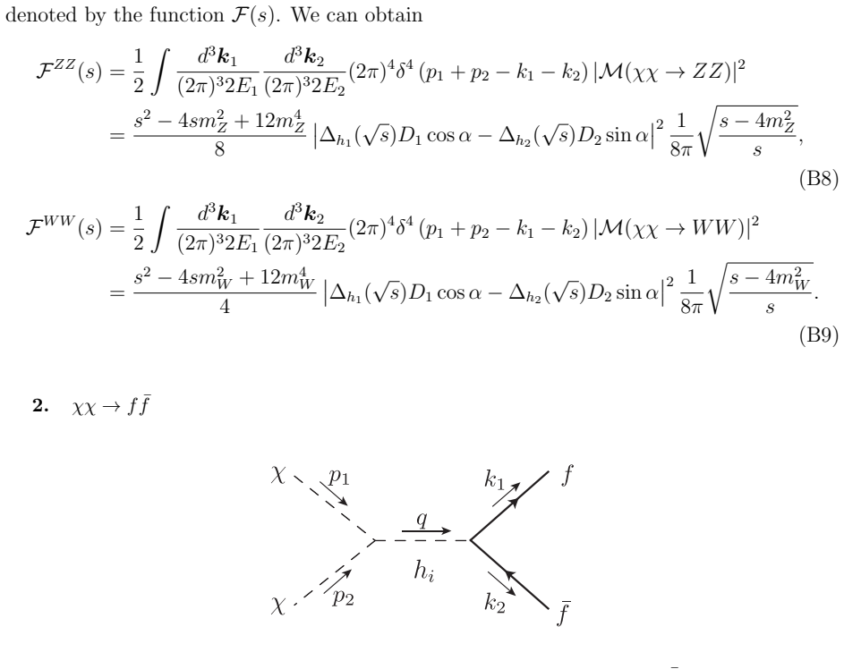
χχ → f ¯f FIG. 8. Feynman diagram of the scattering process χχ → f ¯f . The annihilation into a pair of fermion f and antifermion ¯f is an s-channel process mediated by hi as shown in Fig. 8. The amplitude is given by iM(χχ → f ¯f ) = − i 2 −i mf v φ [i∆h1 (p1 + p2) D1 cos α − i∆h2 (p1 + p2) D2 sin α] ¯ur (k1) vs (k2) , (B10) where ¯u(k1), v(k2) are Dirac...

work page
[7]

3 4 D1λ111φ2 s − m2 h1 s − ¯m2 h1 2 + m2 h1Γ2 h1 + 1 4 D2λ112φ2 s − m2 h2 s − m2 h2 2 + m2 h2Γ2 h2 # + D4 1φ4 8 1 sm2 χ + m2 h1 m2 h1 − 4m2 χ + D2 1φ2 4pk

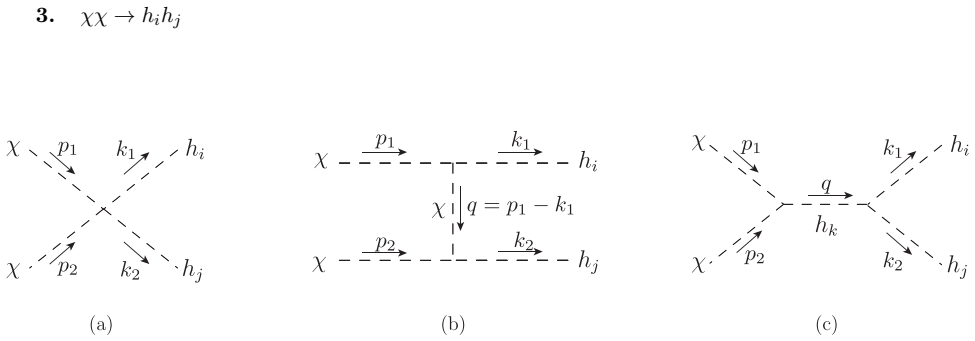
χχ → hihj FIG. 9. Feynman diagram of the scattering process χχ → hihj. The annihilation into a pair of Higgs bosons hi is shown in Fig. 9. The diagrams labeled (a), (b), and (c) correspond to the contact interaction, the t- and u-channel processes, and the s-channel process, respectively. Then, the amplitude is given by iM (χχ → hihj) = iM(a) ij + iM(b) i...

work page
[8]

In the case of vanishing momenta of the incoming particles, it reduces to φ3 (0; m1, m2, m3) ≡ Z 1 0 dx Z 1−x 0 dy 1 (1 − x − y)m2 3 + xm2 1 + ym2 2 = φ3 (0; m2, m1, m3) =    m2 1 log(m2 1/ν2) (m2 1−m2 2)(m2 1−m2

work page

Show all 39 references

[9]

+ m2 2 log(m2 2/ν2) (m2 2−m2 1)(m2 2−m2
[10]

+ m2 3 log(m2 3/ν2) (m2 3−m2 1)(m2 3−m2
[11]

(C20) ν is an arbitrary mass scale

(m1 ̸= m2 ̸= m3 ̸= m1 m2 1 (m2 1−m2 2) 2 log m2 1 m2 2 − 1 m2 1−m2 2 (m1 ̸= m2 = m3) − m2 3 (m2 1−m2 3) 2 log m2 1 m2 3 + 1 m2 1−m2 3 (m1 = m2 ̸= m3) 1 2m2 1 (m1 = m2 = m3) . (C20) ν is an arbitrary mass scale. For this model, ignoring the loops containing the h1-propagator, t...

2000
[12]

Aad et al

G. Aad et al. (ATLAS), Phys. Lett. B 716, 1 (2012), arXiv:1207.7214 [hep-ex]

2012 arXiv
[13]

Chatrchyan et al

S. Chatrchyan et al. (CMS), Phys. Lett. B 716, 30 (2012), arXiv:1207.7235 [hep-ex]

2012 arXiv
[14]

Aad et al

G. Aad et al. (ATLAS), Phys. Rev. D 101, 012002 (2020), arXiv:1909.02845 [hep-ex]

2020 arXiv
[15]

CMS collaboration, CMS-PAS-HIG-19-005 (2020)

2020
[16]

Aalbers et al

J. Aalbers et al. (LZ), (2024), arXiv:2410.17036 [hep-ex]

2024 arXiv
[17]

Barger, P

V. Barger, P. Langacker, M. McCaskey, M. Ramsey-Musolf, and G. Shaughnessy, Phys. Rev. 38 FIG. 15. Effective vertices associated with DM χ when mh2 = 2000 GeV. D 79, 015018 (2009), arXiv:0811.0393 [hep-ph]

2009 arXiv
[18]

Barger, M

V. Barger, M. McCaskey, and G. Shaughnessy, Phys. Rev. D 82, 035019 (2010), arXiv:1005.3328 [hep-ph]

2010 arXiv
[19]

Gonderinger, H

M. Gonderinger, H. Lim, and M. J. Ramsey-Musolf, Phys. Rev. D 86, 043511 (2012), arXiv:1202.1316 [hep-ph]

2012 arXiv
[20]

Coimbra, M

R. Coimbra, M. O. P. Sampaio, and R. Santos, Eur. Phys. J. C 73, 2428 (2013), arXiv:1301.2599 [hep-ph]

2013 arXiv
[21]

Jiang, L

M. Jiang, L. Bian, W. Huang, and J. Shu, Phys. Rev. D 93, 065032 (2016), arXiv:1502.07574 [hep-ph]

2016 arXiv
[22]

Chiang, M

C.-W. Chiang, M. J. Ramsey-Musolf, and E. Senaha, Phys. Rev. D 97, 015005 (2018), 39 arXiv:1707.09960 [hep-ph]

2018 arXiv
[23]

Cheng and L

W. Cheng and L. Bian, Phys. Rev. D 98, 023524 (2018), arXiv:1801.00662 [hep-ph]

2018 arXiv
[24]

Grzadkowski and D

B. Grzadkowski and D. Huang, JHEP 08, 135 (2018), arXiv:1807.06987 [hep-ph]

2018 arXiv
[25]

N. Chen, T. Li, Y. Wu, and L. Bian, Phys. Rev. D 101, 075047 (2020), arXiv:1911.05579 [hep-ph]

2020 arXiv
[26]

G.-C. Cho, C. Idegawa, and E. Senaha, Phys. Lett. B 823, 136787 (2021), arXiv:2105.11830 [hep-ph]

2021 arXiv
[27]

G.-C. Cho, C. Idegawa, and E. Senaha, Phys. Rev. D 106, 115012 (2022), arXiv:2205.12046 [hep-ph]

2022 arXiv
[28]

F. Egle, M. M¨ uhlleitner, R. Santos, and J. a. Viana, (2022), arXiv:2202.04035 [hep-ph]

2022 arXiv
[29]

G.-C. Cho, C. Idegawa, and R. Sugihara, Phys. Lett. B 839, 137757 (2023), arXiv:2212.13029 [hep-ph]

2023 arXiv
[30]

Idegawa and E

C. Idegawa and E. Senaha, Phys. Lett. B 848, 138332 (2024), arXiv:2309.09430 [hep-ph]

2024 arXiv
[31]

G.-C. Cho, C. Idegawa, and R. Inumiya, Nucl. Phys. B 1007, 116688 (2024), arXiv:2312.05776 [hep-ph]

2024 arXiv
[32]

Abe, G.-C

S. Abe, G.-C. Cho, and K. Mawatari, Phys. Rev. D 104, 035023 (2021), arXiv:2101.04887 [hep-ph]

2021 arXiv
[33]

Cho and C

G.-C. Cho and C. Idegawa, Nucl. Phys. B 994, 116320 (2023), arXiv:2304.10096 [hep-ph]

2023 arXiv
[34]

Aghanim et al.(Planck), Astron

N. Aghanim et al.(Planck), Astron. Astrophys. 641, A6 (2020), [Erratum: Astron.Astrophys. 652, C4 (2021)], arXiv:1807.06209 [astro-ph.CO]

2020 arXiv
[35]

Aaboud et al

M. Aaboud et al. (ATLAS), Phys. Lett. B 786, 223 (2018), arXiv:1808.01191 [hep-ex]

2018 arXiv
[36]

Tumasyan et al

A. Tumasyan et al. (CMS), Nature Phys. 18, 1329 (2022), arXiv:2202.06923 [hep-ex]

2022 arXiv
[37]

Khachatryan et al

V. Khachatryan et al. (CMS), Eur. Phys. J. C 74, 3076 (2014), arXiv:1407.0558 [hep-ex]

2014 arXiv
[38]

J. M. Cline, K. Kainulainen, P. Scott, and C. Weniger, Phys. Rev. D 88, 055025 (2013), [Erratum: Phys.Rev.D 92, 039906 (2015)], arXiv:1306.4710 [hep-ph]

2013 arXiv
[39]

Chakraborti, A

S. Chakraborti, A. Milagre, R. Santos, and J. P. Silva, (2025), arXiv:2505.07946 [hep-ph]. 40

2025

Pith tools

Reviewed August 6, 2026 · model on record in the stance chip above.

[1] [1]

Considering a small mixing angle between CP-even scalars to realize a decoupling of the scalar particle from the SM,

work page

[2] [2]

δd (2 + δd) 1 + δd 1 8π3 s 45 2geff(T ) mPl mχ F 4m2 χ # − 1 2 log log

Considering a suppression mechanism such as the degenerate scalar scenario. In fact, when we consider the case α → 0, the scattering amplitude (50) vanishes. On the other hand, the amplitude also disappears when the masses of two scalar particles are degenerate ( mh1 = mh2), and we refer to this suppression mechanism as the degenerate scalar scenario. In ...

work page

[3] [3]

consistency with the latest bounds of the latest LZ experiment [5],

work page

[4] [4]

∂2 ¯m2 i ∂φ2 · m2 i 32π2 log m2 i ¯µ2 − 1 + ∂ ¯m2 i ∂φ 2 · 1 32π2 log m2 i ¯µ2 # , (A6) ∂2VCW ∂φ2 S = X i=h2,χ

reproduction of the observed DM relic abundance, 13 To this end, we perform a parameter scan over the following ranges: 10 ≤ vs GeV ≤ 1000 − 5003 ≤ a1/GeV3 ≤ 0 125 ≤ mχ GeV ≤ 5000. (64) As seen in Eq. (6), ensuringφS > 0 typically requires a1 < 0. Therefore, we focus on negative values of a1 in this analysis. For the second scalar mass mh2, we consider fo...

work page 2000

[5] [5]

χχ → V V The annihilation into a pair of gauge bosons Z, Wis an s-channel process mediated by hi as shown in Fig. 7. The amplitudes are given by iM(χχ → ZZ ) = m2 Zφ2 v2 (i∆h1 (p1 + p2) D1 cos α − i∆h2 (p1 + p2) D2 sin α) gµνϵ(r) µ (k1) ϵ(s) µ (k2) , (B1) iM(χχ → W W) = m2 W φ2 v2 (i∆h1 (p1 + p2) D1 cos α − i∆h2 (p1 + p2) D2 sin α) gµνϵ(r) µ (k1) ϵ(s) µ (...

work page

[6] [6]

χχ → f ¯f FIG. 8. Feynman diagram of the scattering process χχ → f ¯f . The annihilation into a pair of fermion f and antifermion ¯f is an s-channel process mediated by hi as shown in Fig. 8. The amplitude is given by iM(χχ → f ¯f ) = − i 2 −i mf v φ [i∆h1 (p1 + p2) D1 cos α − i∆h2 (p1 + p2) D2 sin α] ¯ur (k1) vs (k2) , (B10) where ¯u(k1), v(k2) are Dirac...

work page

[7] [7]

3 4 D1λ111φ2 s − m2 h1 s − ¯m2 h1 2 + m2 h1Γ2 h1 + 1 4 D2λ112φ2 s − m2 h2 s − m2 h2 2 + m2 h2Γ2 h2 # + D4 1φ4 8 1 sm2 χ + m2 h1 m2 h1 − 4m2 χ + D2 1φ2 4pk

χχ → hihj FIG. 9. Feynman diagram of the scattering process χχ → hihj. The annihilation into a pair of Higgs bosons hi is shown in Fig. 9. The diagrams labeled (a), (b), and (c) correspond to the contact interaction, the t- and u-channel processes, and the s-channel process, respectively. Then, the amplitude is given by iM (χχ → hihj) = iM(a) ij + iM(b) i...

work page

[8] [8]

In the case of vanishing momenta of the incoming particles, it reduces to φ3 (0; m1, m2, m3) ≡ Z 1 0 dx Z 1−x 0 dy 1 (1 − x − y)m2 3 + xm2 1 + ym2 2 = φ3 (0; m2, m1, m3) =    m2 1 log(m2 1/ν2) (m2 1−m2 2)(m2 1−m2

work page