REVIEW 2 major objections 4 minor 1 cited by
A Structured Proximal Stochastic Variance Reduced Zeroth-order Algorithm
T0 review · 2 major / 4 minor · reviewed 2026-08-06 · deepseek-v4-flash
Pith's one-line read The paper introduces VR-SZD, a variance-reduced zeroth-order proximal algorithm that estimates gradients with forward finite differences along $\ell \le d$ random orthogonal directions, and proves it matches the best known $O(d n^{2/3}…
desk verdict A clean, competent paper that closes a real gap in variance-reduced zeroth-order optimization; the advertised O(d n^{2/3}/ε) rate is internally consistent, with two caveats worth noting. read the letter →
The pith
A machine-rendered reading of the paper's core claim, the machinery that carries it, and where it could break.
The reading
What carries the argument
The engine is the structured stochastic gradient estimator $\hat{g}_i(x,G,\beta) = \frac{d}{\ell}\sum_{j=1}^\ell \frac{f_i(x+\beta G e_j)-f_i(x)}{\beta} G e_j$, with $G$ uniform on the orthogonal group $O(d)$ and $\ell \le d$ directions. Lemma 4 shows that this estimator is unbiased for the gradient of the smoothed function $f_\beta(x)=\mathbb{E}_{u\sim U(\mathbb{B}^d)}[f(x+\beta u)]$, which turns a finite-difference direction into a controllable surrogate; Lemma 8 then bounds the variance of the SVRG direction $v^\tau_k$ by a drift term plus a term proportional to $\beta_\tau^2$. The proof is carried by a Lyapunov function $R^\tau_k = F(x^\tau_k) + c_k\|x^\tau_k - x^\tau_0\|^2$ that absorbs the inner-loop drift, and stationarity is measured through the proximal gradient mapping $G_\gamma(x)=\gamma^{-1}(x - \mathrm{prox}_{\gamma h}(x-\gamma\nabla f(x)))$.
What would settle it
Take a family of non-convex finite sums whose components are $L$-smooth but with gradients that vary rapidly at scale $\beta$, run VR-SZD with $b=\lceil n^{2/3}\rceil$, $m=\lceil \sqrt{b}\rceil$, $\ell=\lceil d/c\rceil$, and record the number of function evaluations needed to drive $\mathbb{E}\|G_\gamma(x)\|^2$ below a fixed $\varepsilon$; if the scaling in $n$ is worse than $n^{2/3}$, or an extra $\varepsilon^{-2}$ factor appears, the central complexity claim is wrong.
Extended reading notes
Core claim
The paper's central claim is that orthogonal structure in the stochastic finite-difference estimator is free: VR-SZD attains a function-evaluation complexity of $O(d n^{2/3}\varepsilon^{-1})$ for non-convex composite finite-sum minimization, matching the best known zeroth-order finite-sum rates, while using only $\ell \le d$ directions per stochastic gradient estimate and forward rather than central differences. Under the revised Polyak-Łojasiewicz condition, Theorem 2 gives $\mathbb{E}[F(x_0^{\tau+1})-\min F] \le \alpha^{m(\tau+1)}[\mathbb{E}[F(x_0^\tau)-\min F] + \text{(error term)}$, with an overall complexity $O((nd/(\gamma\mu m) + b\ell/(\gamma\mu))\log(1/\varepsilon))$. These results hold in the composite setting where $h$ is convex and proximable, and they avoid the bounded stochastic-gradient variance assumption used by earlier composite zeroth-order analyses.
Load-bearing premise
The rates depend on every one of the $n$ component functions being smooth, meaning each has a derivative whose length changes at most proportionally to distance, and on the nonsmooth part $h$ being convex and easy to project onto; if a component is nonsmooth or has unbounded gradient variation, the finite-difference bias and variance bounds in the proof no longer hold.
Editorial extensions
If this is right
- With $b=\lceil n^{2/3}\rceil$, $m=\lceil \sqrt{b}\rceil$, and $\ell=\lceil d/c\rceil$, VR-SZD reaches $\mathbb{E}\|G_\gamma(x)\|^2 \le \varepsilon$ in $O(d n^{2/3}\varepsilon^{-1})$ function evaluations for non-convex composite finite sums.
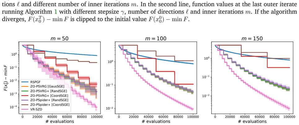
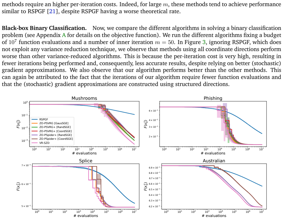
- Each outer iteration costs $n(d+1)+2mb(\ell+1)$ function evaluations, so for $\ell < d$ the per-iteration cost is lower than coordinate-direction variants such as ZO-PSVRG+ with CoordSGE and ZO-PSpider+ with CoordSGE.
- Under the revised Polyak-Łojasiewicz condition, choosing a square-summable discretization sequence makes VR-SZD converge exponentially fast to a global minimizer, while a constant discretization gives linear convergence to a neighborhood of size proportional to $\beta^2$.
- The convergence metric is the proximal gradient mapping, so the rates apply to composite problems with a nonsmooth convex and proximable part $h$, not only to smooth objectives.
- Choosing $\ell=1$ recovers the inner iteration of a prior hybrid zeroth-order method as a special case, while using cheaper forward differences in the outer full-gradient surrogate.
Reading between the lines
- The paper fixes $\ell$ and tunes it by grid search, but its own experiments show a budget-dependent optimal number of directions; an adaptive schedule that grows $\ell$ as outer iterates stabilize is a natural, testable extension.
- Because the outer full-gradient surrogate costs $d$ evaluations regardless of $\ell$, VR-SZD is most attractive when $d$ is moderate enough for the outer pass but too large to pay $d$ directions on every inner step; black-box adversarial perturbation and LLM fine-tuning budgets are the settings to check, which the paper does not run.
- Replacing the forward-difference full gradient by a central-difference version would trade $d$ extra outer evaluations for smaller bias constants, and the same Lyapunov machinery should carry through, so a direct comparison of the two discretization choices is a close-by experiment.
Editorial analysis
A structured set of objections, weighed in public.
Referee Report
Summary. The paper proposes VR-SZD, a variance-reduced zeroth-order proximal algorithm for composite finite-sum minimization of the form min_x f(x)+h(x), where f is an average of differentiable but potentially nonconvex components and h is convex, nonsmooth, and proximable. The algorithm uses forward finite differences along the full coordinate basis to estimate the full gradient at each outer iteration and along a set of ℓ random orthogonal directions to estimate stochastic gradients in inner iterations. The main theoretical results are a nonconvex convergence rate in terms of the gradient mapping with function-evaluation complexity O(d n^{2/3} ε^{-1}) for a specific parameter choice, and a linear convergence rate under a revised Polyak-Łojasiewicz condition. Numerical experiments on LASSO and binary classification compare VR-SZD favorably with existing zeroth-order variance-reduced methods.
Significance. If the advertised rates hold, this is a useful contribution: it extends structured (orthogonal-direction) zeroth-order estimators to variance-reduced proximal finite-sum methods, uses cheaper forward differences than the central-difference estimators in several prior works, and matches the best known finite-sum complexity O(d n^{2/3} ε^{-1}) while handling a nonsmooth proximable term h. The proofs are unusually detailed, with explicit constants and parameter choices rather than asymptotic hand-waving, and the algorithm is clearly positioned against the prior work of Ji et al., Kazemi and Wang, Huang et al., and the authors' own structured zeroth-order papers. The numerical study is reasonable and the plots are informative. The main caveat is that the headline complexity requires ℓ=Θ(d), so the 'lower per-iteration cost' framing is weaker than the abstract suggests for bounded ℓ.
major comments (2)
- [Section 3.1, Theorem 1 and Corollary 1] The step-size condition printed in Theorem 1 and the step-size chosen in Corollary 1 are not compatible as written. If the second term in the theorem's min is read as sqrt(ℓb)/(sqrt(32(e−1)) d L m), then for d≥2 the corollary's choice γ=sqrt(ℓb)/(10 L m sqrt(d)) exceeds it (for d=2 the ratio is about 1.05), so Corollary 1 cannot be deduced from Theorem 1. If, instead, the denominator is meant to be sqrt(32(e−1)d) L m, the display should say so, because the current rendering is ambiguous. The proof in Appendix D actually uses the condition γ<sqrt(ℓb)/(sqrt(32(e−1)d) L m) to make the coefficient before eq. (23) negative. Please correct the theorem statement or prove Corollary 1 directly from the proof's condition. This is load-bearing because Corollary 1(iii) is the advertised O(d n^{2/3} ε^{-1}) complexity.
- [Section 3.1, Corollary 1(i)] The displayed constant (2α+2)/(2α+1) is not a valid upper bound for sum_{τ=0}^T (τ+1)^{-2α} for all α>1/2; for α=1 the sum tends to ζ(2)=π²/6≈1.645, which is larger than 4/3. The asymptotic O(1/T) conclusion is still correct, since the partial sums are bounded by ζ(2α), but the explicit constant should be replaced (e.g., by ζ(2α)) or the inequality justified.
minor comments (4)
- [Abstract and Section 2] The abstract says 'non-smooth finite-sum minimization,' but Assumption 1 requires every component f_i to be differentiable with L-Lipschitz gradient; only h may be nonsmooth. This is explicit in Section 2 and matches the literature, but the terminology should be adjusted to avoid overstating the scope.
- [Section 3.1, Discussion] The claim of 'lower per-iteration costs' should be qualified: matching the O(d n^{2/3} ε^{-1}) complexity requires ℓ=ceil(d/c), i.e., ℓ=Θ(d). With ℓ=1 the displayed complexity becomes O(d^{3/2} n^{2/3} ε^{-1}), which is worse than the coordinate-direction baselines, so the advantage is specifically for the structured ℓ=Θ(d) regime.
- [Appendix C, Lemma 8 proof] In the proof of Lemma 8, the notation EG^τ_k is used inconsistently with the conditional expectation notation defined at the start of Appendix C; this is cosmetic but makes the proof harder to follow.
- [Appendix D, proof of Corollary 2(i)] The displayed equality between the expression with sum η_i² and the closed form with (1−α^{m(τ+1)})/(1−α^m) is not an equality; it should be an inequality. The final bound is still correct, but the line should be fixed.
Circularity Check
No significant circularity: the advertised convergence rates are derived from explicit assumptions via self-contained smoothing and variance-reduction arguments; parameter choices are balancing steps in the proven bounds, not fitted predictions.
full rationale
The derivation chain is self-contained and does not reduce to its inputs. The structured estimator (eq. 4) is shown unbiased for the smoothed gradient in Lemma 4, with smoothing inequalities quoted from standard sources (e.g., [17, Proposition 7.5]) and re-proved dependence in Proposition 1. The bias/variance controls in Lemmas 7 and 8 follow from L-smoothness of the component functions under Assumption 1, and the non-convex rate in Theorem 1 is obtained by a Lyapunov telescoping argument over the inner and outer iterations. Corollary 1's parameter choices are explicit balancing decisions: the stepsize γ=√(ℓb)/(10Lm√d), the discretization βτ, and the count choices b=ceil(n^{2/3}), m=ceil(√b), ℓ=ceil(d/c) are substituted into the theorem's bound to make the error ≤ε. Nothing is fitted to data and then renamed a prediction. The revised Polyak-Łojasiewicz result (Theorem 2, Corollary 2) likewise follows from Assumptions 1–2 using the same estimator bounds and a standard contraction argument; the RPL condition is attributed to external prior work [31,37], not to the authors' own unpublished results. Self-citations to [34,54,56,55] appear in the introduction and related work as contextual claims or motivation (e.g., that orthogonal directions often perform better), not as load-bearing steps in the proofs; the proofs themselves re-derive the needed lemmas or cite external standard references [17,31,43]. The broadened 'non-smooth finite-sum minimization' phrasing is tempered by Assumption 1, which requires each fi to be L-smooth and permits nonsmoothness only in h; this is a scope limitation, not circular reasoning. The advertised O(d n^{2/3}/ε) rate also requires ℓ=Θ(d), a caveat about per-iteration cost but not a circularity. No step was found in which a claimed result equals an input by construction, and no load-bearing self-citation chain forces the conclusions.
Assumptions & free parameters
free parameters (5)
- stepsize γ =
grid search in experiments; theory requires γ < min{1/(4L), sqrt(ℓb)/(sqrt(32(e-1)d) L m)}
- smoothing parameter βτ =
βτ = β/d (τ+1)^{-α} or constant β in corollaries; βτ ∈ {1e-5, 1e-7} in experiments
- batch size b =
b = ceil(n^{2/3}) in Corollary 1(iii); b = 1 in experiments
- inner iterations m =
m = ceil(sqrt(b)) in theory; m ∈ {50, 100, 150} in experiments
- number of directions ℓ =
ℓ = ceil(d/c) in theory; ℓ ∈ {1, 10, 25, 50} in experiments
assumptions (5)
- domain assumption Each f_i is L-smooth and h is convex and proximable (Assumption 1).
- domain assumption F satisfies the revised Polyak-Łojasiewicz condition with gradient mapping (Assumption 2).
- standard math Standard measure-theoretic lemmas: normalized Haar measure on O(d), spherical measure, and the pushforward result in Lemma 3.
- standard math Classical smoothing and descent lemmas, including Proposition 1 and Lemma 5.
- domain assumption Exact, noiseless function value queries are available.
Cite this review
Pith. "Pith review of A Structured Proximal Stochastic Variance Reduced Zeroth-order Algorithm." pith.science (2026). https://pith.science/paper/I4SQC6M5
@misc{pith2026250623758,
  author       = {Pith},
  title        = {Pith review of: A Structured Proximal Stochastic Variance Reduced Zeroth-order Algorithm},
  year         = {2026},
  howpublished = {\url{https://pith.science/paper/I4SQC6M5}},
  note         = {Machine review of arXiv:2506.23758}
}
read the original abstract
Minimizing finite sums of functions is a central problem in optimization, arising in numerous practical applications. Such problems are commonly addressed using first-order optimization methods. However, these procedures cannot be used in settings where gradient information is unavailable. Finite-difference methods provide an alternative by approximating gradients through function evaluations along a set of directions. For finite-sum minimization problems, it was shown that incorporating variance-reduction techniques into finite-difference methods can improve convergence rates. Additionally, recent studies showed that imposing structure on the directions (e.g., orthogonality) enhances performance. However, the impact of structured directions on variance-reduced finite-difference methods remains unexplored. In this work, we close this gap by proposing a structured variance-reduced finite-difference algorithm for non-smooth finite-sum minimization. We analyze the proposed method, establishing convergence rates for non-convex functions and those satisfying the Polyak-{\L}ojasiewicz condition. Our results show that our algorithm achieves state-of-the-art convergence rates while incurring lower per-iteration costs. Finally, numerical experiments highlight the strong practical performance of our method.
Figures

Forward citations
Cited by 1 Pith paper
-
Langevin for Nonconvex Optimization: Exact, Inexact and Zeroth-Order
For smooth dissipative nonconvex objectives, exact, inexact and zeroth-order ULA achieve expected excess risk ε with iteration complexity ~O~(β²dC_LS²/ε²) and zeroth-order evaluation complexity ~O~(β⁴d³C_LS³/ε⁴).
Reference graph
Works this paper leans on
- [24]
-
[1]
A. S. Berahas, L. Cao, K. Choromanski, and K. Scheinberg. A theoretical and empirical comparison of gradient approximations in derivative-free optimization. Foundations of Computational Mathematics, 22(2):507–560, 2022
work page 2022
-
[2]
D. P. Bertsekas. Stochastic optimization problems with nondifferentiable cost functionals. Journal of Optimization Theory and Applications, 12(2):218–231, Aug 1973
work page 1973
- [3]
-
[4]
H. Cai, Y. Lou, D. Mckenzie, and W. Yin. A zeroth-order block coordinate descent algorithm for huge- scale black-box optimization. In Proceedings of the 38th International Conference on Machine Learning , volume 139 of Proceedings of Machine Learning Research, pages 1193–1203, 18–24 Jul 2021
work page 2021
-
[5]
H. Cai, D. McKenzie, W. Yin, and Z. Zhang. Zeroth-order regularized optimization (zoro): Approximately sparse gradients and adaptive sampling. SIAM Journal on Optimization, 32(2):687–714, 2022
work page 2022
-
[6]
C. C. Chang and C. J. Lin. Libsvm: A library for support vector machines.ACM Trans. Intell. Syst. Technol., 2(3), May 2011
work page 2011
-
[7]
Randomized Derivative-Free Optimization of Noisy Convex Functions
R. Chen and S. Wild. Randomized derivative-free optimization of noisy convex functions. arXiv preprint arXiv:1507.03332, 2015
work page Pith review arXiv 2015
Show all 79 references
-
[8]
Y. Chikuse. Statistics on special manifolds, volume 174. 2012
2012
-
[9]
Choromanski, M
K. Choromanski, M. Rowland, V. Sindhwani, R. Turner, and A. Weller. Structured evolution with compact architectures for scalable policy optimization. In Jennifer Dy and Andreas Krause, editors, Proceedings of the 35th International Conference on Machine Learning , volume 80 of...
2018
-
[10]
A. R. Conn, K. Scheinberg, and L. N. Vicente. Introduction to Derivative-Free Optimization . Society for Industrial and Applied Mathematics, 2009
2009
-
[11]
Defazio, F
A. Defazio, F. Bach, and S. Lacoste-Julien. Saga: A fast incremental gradient method with support for non-strongly convex composite objectives. In Z. Ghahramani, M. Welling, C. Cortes, N. Lawrence, and K.Q. Weinberger, editors, Advances in Neural Information Processing Systems...
2014
-
[12]
Demetrio, B
L. Demetrio, B. Biggio, G. Lagorio, F. Roli, and A. Armando. Functionality-preserving black-box optimiza- tion of adversarial windows malware. IEEE Transactions on Information Forensics and Security, 2021
2021
-
[13]
J. C. Duchi, M. I. Jordan, M. J. Wainwright, and A. Wibisono. Optimal rates for zero-order convex opti- mization: The power of two function evaluations. IEEE Transactions on Information Theory, 61(5):2788– 2806, 2015
2015
-
[14]
C. Fang, C. J. Li, Z. Lin, and T. Zhang. Spider: Near-optimal non-convex optimization via stochastic path-integrated differential estimator. In S. Bengio, H. Wallach, H. Larochelle, K. Grauman, N. Cesa- Bianchi, and R. Garnett, editors, Advances in Neural Information Processin...
2018
-
[15]
Flaxman, A
A. Flaxman, A. Tauman Kalai, and B. McMahan. Online convex optimization in the bandit setting: Gra- dient descent without a gradient. In SODA ’05 Proceedings of the sixteenth annual ACM-SIAM symposium on Discrete algorithms, pages 385–394, January 2005
2005
-
[16]
P. I. Frazier. Bayesian Optimization, chapter 11, pages 255–278. INFORMS, 2018. 14
2018
-
[17]
X. Gao, B. Jiang, and S. Zhang. On the information-adaptive variants of the admm: An iteration com- plexity perspective. Journal of Scientific Computing, 76(1):327–363, Jul 2018
2018
-
[18]
Gasnikov, A
A. Gasnikov, A. Novitskii, V. Novitskii, F. Abdukhakimov, D. Kamzolov, A. Beznosikov, M. Takac, P. Dvurechensky , and B. Gu. The power of first-order smooth optimization for black-box non-smooth problems. In Kamalika Chaudhuri, Stefanie Jegelka, Le Song, Csaba Szepesvari, Gang...
2022
-
[19]
Gautam, Y
T. Gautam, Y. Park, H. Zhou, P. Raman, and W. Ha. Variance-reduced zeroth-order methods for fine- tuning language models. In Ruslan Salakhutdinov, Zico Kolter, Katherine Heller, Adrian Weller, Nuria Oliver, Jonathan Scarlett, and Felix Berkenkamp, editors,Proceedings of the 41...
2024
-
[20]
Ghadimi and G
S. Ghadimi and G. Lan. Stochastic first- and zeroth-order methods for nonconvex stochastic program- ming. SIAM Journal on Optimization, 23(4):2341–2368, 2013
2013
-
[21]
Ghadimi, G
S. Ghadimi, G. Lan, and H. Zhang. Mini-batch stochastic approximation methods for nonconvex stochas- tic composite optimization. Mathematical Programming, 155(1):267–305, Jan 2016
2016
-
[22]
C. Guo, J. Gardner, Y. You, A. G. Wilson, and K. Weinberger. Simple black-box adversarial attacks. In Kamalika Chaudhuri and Ruslan Salakhutdinov, editors, Proceedings of the 36th International Conference on Machine Learning, volume 97 of Proceedings of Machine Learning Resear...
2019
-
[23]
C. R. Harris, K. J. Millman, S. J. van der Walt, R. Gommers, P. Virtanen, D. Cournapeau, E. Wieser, J. Taylor, S. Berg, N. J. Smith, R. Kern, M. Picus, S. Hoyer, M. H. van Kerkwijk, M. Brett, A. Haldane, J. Fern´andez del R´ıo, M. Wiebe, P. Peterson, P. G´erard-Marchant, K. Sh...
2020
-
[25]
Huang, L
F. Huang, L. Tao, and S. Chen. Accelerated stochastic gradient-free and projection-free methods. In Hal Daum ´e III and Aarti Singh, editors, Proceedings of the 37th International Conference on Machine Learning, volume 119 of Proceedings of Machine Learning Research, pages 451...
2020
-
[26]
J. D. Hunter. Matplotlib: A 2d graphics environment. Computing in Science & Engineering , 9(3):90–95, 2007
2007
-
[27]
Ilyas, L
A. Ilyas, L. Engstrom, A. Athalye, and J. Lin. Black-box adversarial attacks with limited queries and information. In Jennifer Dy and Andreas Krause, editors, Proceedings of the 35th International Conference on Machine Learning, volume 80 of Proceedings of Machine Learning Res...
2018
-
[28]
S. J. Reddi, S. Sra, B. Poczos, and A. J. Smola. Proximal stochastic methods for nonsmooth nonconvex finite-sum optimization. In D. Lee, M. Sugiyama, U. Luxburg, I. Guyon, and R. Garnett, editors,Advances in Neural Information Processing Systems, volume 29. Curran Associates, ...
2016
-
[29]
K. Ji, Z. Wang, Y. Zhou, and Y. Liang. Improved zeroth-order variance reduced algorithms and analysis for nonconvex optimization. In Kamalika Chaudhuri and Ruslan Salakhutdinov, editors, Proceedings of the 36th International Conference on Machine Learning , volume 97 of Procee...
2019
-
[30]
Johnson and T
R. Johnson and T. Zhang. Accelerating stochastic gradient descent using predictive variance reduction. In C.J. Burges, L. Bottou, M. Welling, Z. Ghahramani, and K.Q. Weinberger, editors, Advances in Neural Information Processing Systems, volume 26. Curran Associates, Inc., 2013
2013
-
[31]
Kazemi and L
E. Kazemi and L. Wang. Efficient zeroth-order proximal stochastic method for nonconvex nonsmooth black-box problems. Machine Learning, 113(1):97–120, Jan 2024
2024
-
[32]
Kozak, S
D. Kozak, S. Becker, A. Doostan, and L. Tenorio. Stochastic subspace descent. arXiv preprint arXiv:1904.01145, 2019
1904 arXiv
-
[33]
Kozak, S
D. Kozak, S. Becker, A. Doostan, and L. Tenorio. A stochastic subspace approach to gradient-free opti- mization in high dimensions. Computational Optimization and Applications, 79(2):339–368, Jun 2021
2021
-
[34]
Kozak, C
D. Kozak, C. Molinari, L. Rosasco, L. Tenorio, and S. Villa. Zeroth-order optimization with orthogonal random directions. Mathematical Programming, 199(1):1179–1219, May 2023
2023
-
[35]
Lankham, B
I. Lankham, B. Nachtergaele, and A. Schilling. Linear Algebra as an Introduction to Abstract Mathematics. WORLD SCIENTIFIC, 2016
2016
-
[36]
R. M. Lewis, V. Torczon, and M. W. Trosset. Direct search methods: then and now. Journal of Computa- tional and Applied Mathematics, 124(1):191–207, 2000. Numerical Analysis 2000. Vol. IV: Optimization and Nonlinear Equations
2000
-
[37]
Li and J
Z. Li and J. Li. A simple proximal stochastic gradient method for nonsmooth nonconvex optimization. In S. Bengio, H. Wallach, H. Larochelle, K. Grauman, N. Cesa-Bianchi, and R. Garnett, editors, Advances in Neural Information Processing Systems, volume 31. Curran Associates, I...
2018
-
[38]
T. Lin, Z. Zheng, and M. Jordan. Gradient-free methods for deterministic and stochastic nonsmooth nonconvex optimization. In S. Koyejo, S. Mohamed, A. Agarwal, D. Belgrave, K. Cho, and A. Oh, editors, Advances in Neural Information Processing Systems , volume 35, pages 26160–2...
2022
-
[39]
L. Liu, M. Cheng, C. J. Hsieh, and D. Tao. Stochastic zeroth-order optimization via variance reduction method. arXiv preprint arXiv:1805.11811, 2018
2018 arXiv
-
[40]
S. Liu, B. Kailkhura, P. Chen, P. Ting, S. Chang, and L. Amini. Zeroth-order stochastic variance reduction for nonconvex optimization. In Advances in Neural Information Processing Systems, volume 31, 2018
2018
-
[41]
Lojasiewicz
S. Lojasiewicz. A topological property of real analytic subsets. Coll. du CNRS, Les ´equations aux d´eriv´ees partielles, 117(87-89):2, 1963
1963
-
[42]
Malladi, T
S. Malladi, T. Gao, E. Nichani, A. Damian, J. D. Lee, D. Chen, and S. Arora. Fine-tuning language models with just forward passes. In Advances in Neural Information Processing Systems, volume 36, 2023
2023
-
[43]
P. Mattila. Geometry of Sets and Measures in Euclidean Spaces: Fractals and Rectifiability . Cambridge Studies in Advanced Mathematics. Cambridge University Press, 1995
1995
-
[44]
Mezzadri
F. Mezzadri. How to generate random matrices from the classical compact groups. arXiv preprint math- ph/0609050, 2006
2006
-
[45]
Moosavi-Dezfooli, A
S. Moosavi-Dezfooli, A. Fawzi, O. Fawzi, and P. Frossard. Universal adversarial perturbations. InProceed- ings of the IEEE Conference on Computer Vision and Pattern Recognition (CVPR), July 2017
2017
-
[46]
H. Mu, Y. Tang, and Z. Li. Variance-reduced gradient estimator for nonconvex zeroth-order distributed optimization, 2024
2024
-
[47]
Nesterov and V
Y. Nesterov and V. Spokoiny . Random gradient-free minimization of convex functions. Foundations of Computational Mathematics, 17:527–566, 2017. 16
2017
-
[48]
Paszke, S
A. Paszke, S. Gross, F. Massa, A. Lerer, J. Bradbury , G. Chanan, T. Killeen, Z. Lin, N. Gimelshein, L. Antiga, A. Desmaison, A. Kopf, E. Yang, Z. DeVito, M. Raison, A. Tejani, S. Chilamkurthy , B. Steiner, L. Fang, J. Bai, and S. Chintala. PyTorch: An imperative style, high-p...
2019
-
[49]
B. T. Polyak. Introduction to optimization. Optimization Software Inc., Publications Division, New York , 1:32, 1987
1987
-
[50]
Pougkakiotis and D
S. Pougkakiotis and D. Kalogerias. A zeroth-order proximal stochastic gradient method for weakly convex stochastic optimization. SIAM Journal on Scientific Computing, 45(5):A2679–A2702, 2023
2023
-
[51]
Raffel, N
C. Raffel, N. Shazeer, A. Roberts, K. Lee, S. Narang, M. Matena, Y. Zhou, W. Li, and P. J. Liu. Exploring the limits of transfer learning with a unified text-to-text transformer.J. Mach. Learn. Res., 21(1), January 2020
2020
-
[52]
Rando, L
M. Rando, L. Carratino, S. Villa, and L. Rosasco. Ada-bkb: Scalable gaussian process optimization on continuous domains by adaptive discretization. In Proceedings of The 25th International Conference on Artificial Intelligence and Statistics, volume 151, 28–30 Mar 2022
2022
-
[53]
Rando, L
M. Rando, L. Demetrio, L. Rosasco, and F. Roli. A new formulation for zeroth-order optimization of adversarial exemples in malware detection, 2024
2024
-
[54]
Rando, C
M. Rando, C. Molinari, L. Rosasco, and S. Villa. An optimal structured zeroth-order algorithm for non- smooth optimization. In A. Oh, T. Naumann, A. Globerson, K. Saenko, M. Hardt, and S. Levine, editors, Advances in Neural Information Processing Systems , volume 36, pages 367...
2023
-
[55]
Rando, C
M. Rando, C. Molinari, L. Rosasco, and S. Villa. A structured tour of optimization with finite differences, 2025
2025
-
[56]
Rando, C
M. Rando, C. Molinari, S. Villa, and L. Rosasco. Stochastic zeroth order descent with structured direc- tions. Computational Optimization and Applications, Oct 2024
2024
-
[57]
S. J. Reddi, A. Hefny , S. Sra, B. Poczos, and A. Smola. Stochastic variance reduction for nonconvex opti- mization. In Maria Florina Balcan and Kilian Q. Weinberger, editors,Proceedings of The 33rd International Conference on Machine Learning, volume 48 of Proceedings of Mach...
2016
-
[58]
Salimans, J
T. Salimans, J. Ho, X. Chen, S. Sidor, and I. Sutskever. Evolution strategies as a scalable alternative to reinforcement learning, 2017
2017
-
[59]
Sartore, M
C. Sartore, M. Rando, G. Romualdi, C. Molinari, L. Rosasco, and D. Pucci. Automatic gain tuning for humanoid robots walking architectures using gradient-free optimization techniques, 2024
2024
-
[60]
O. Shamir. An optimal algorithm for bandit and zero-order convex optimization with two-point feedback. The Journal of Machine Learning Research, 18(1):1703–1713, 2017
2017
-
[61]
C. Totzeck. Trends in Consensus-Based Optimization, pages 201–226. Springer International Publishing, Cham, 2022
2022
-
[62]
Traor ´e, V
C. Traor ´e, V. Apidopoulos, S. Salzo, and S. Villa. Variance reduction techniques for stochastic proximal point algorithms. Journal of Optimization Theory and Applications, 203(2):1910–1939, Nov 2024
1910
-
[63]
S. Wang, Y. Shi, and Y. Han. Universal perturbation generation for black-box attack using evolutionary algorithms. In 2018 24th International Conference on Pattern Recognition (ICPR), pages 1277–1282, 2018
2018
-
[64]
Wang and Y
T. Wang and Y. Feng. Convergence rates of zeroth order gradient descent for łojasiewicz functions. INFORMS Journal on Computing, Mar 2024. 17
2024
-
[65]
Zhang, P
Y. Zhang, P. Li, J. Hong, J. Li, Y. Zhang, W. Zheng, P. Chen, J. D. Lee, W. Yin, M. Hong, Z. Wang, S. Liu, and T. Chen. Revisiting zeroth-order optimization for memory-efficient LLM fine-tuning: A benchmark. In Proceedings of the 41st International Conference on Machine Learni...
2024
-
[66]
Zhu and M
Y. Zhu and M. Zhang. An adaptive variance reduction zeroth-order algorithm for finite-sum optimization. Frontiers in Computing and Intelligent Systems, 3(3):66–70, May 2023. 18 A Experimental Details In this appendix, we provide the details of the experiments presented in Sect...
2023
-
[67]
fi(x + βv) − fi(x) − ⟨∇fi(x), βv⟩ !2# + 3 d2 ℓβ2 EiEv
Moreover, with the following Lemma, we show that the gradient of the smooth approximation fβ can be expressed as an expectation of the surrogate in eq. (4). Lemma 4 (Smoothing Lemma). Let (Ω, F , P) and (Ω′, F ′, P′) be probability spaces. Let G : Ω → O(d) and i : Ω ′ → [n] be...
-
[68]
Noticing that F (xT +1 0 ) ≥ min F and dividing by ∆γm(T + 1), we conclude the proof: 1 (T + 1)m TX τ =0 m−1X k=0 E ∥Gγ(xτ k)∥2 ≤ E F (x0
− F (xT +1 0 ) + C1mγ TX τ =0 β2 τ . Noticing that F (xT +1 0 ) ≥ min F and dividing by ∆γm(T + 1), we conclude the proof: 1 (T + 1)m TX τ =0 m−1X k=0 E ∥Gγ(xτ k)∥2 ≤ E F (x0
-
[69]
Proof of Corollary 1 From Theorem 1, choosing the stepsize γ <min( 1 4L , √ ℓb 10Lm √ d ), we have 1 (T + 1)m TX τ =0 m−1X k=0 E ∥Gγ(xτ k)∥2 ≤ 10L √ d√ ℓb F (x0
− min F ∆γm(T + 1) + C1 ∆(T + 1) TX τ =0 β2 τ . Proof of Corollary 1 From Theorem 1, choosing the stepsize γ <min( 1 4L , √ ℓb 10Lm √ d ), we have 1 (T + 1)m TX τ =0 m−1X k=0 E ∥Gγ(xτ k)∥2 ≤ 10L √ d√ ℓb F (x0
-
[70]
Note that, due to the choice of the stepsize, ∆ ≥ 1
− min F ∆(T + 1) + 3d ℓb + 2 + 3d L2d ∆(T + 1) TX τ =0 β2 τ . Note that, due to the choice of the stepsize, ∆ ≥ 1
-
[71]
Thus, 1 (T + 1)m TX τ =0 m−1X k=0 E ∥Gγ(xτ k)∥2 ≤ 40L √ d√ ℓb F (x0
-
[72]
(24) Points (i) and (ii) can be proved by replacing the corresponding value of βτ in eq
− min F T + 1 + 4 3d ℓb + 2 + 3d L2d T + 1 TX τ =0 β2 τ . (24) Points (i) and (ii) can be proved by replacing the corresponding value of βτ in eq. (24). Indeed, with the choice (i), we have βτ = β d (τ + 1)−α with α >1/2. Thus, we get 1 (T + 1)m TX τ =0 m−1X k=0 E ∥Gγ(xτ k)∥2 ...
-
[73]
28 Instead, with the choice βτ = β d (ii) we get 1 (T + 1)m TX τ =0 m−1X k=0 E ∥Gγ(xτ k)∥2 ≤ 40L √ d√ ℓb F (x0
− min F T + 1 + 4 3d ℓb + 2 + 3d 2α + 2 2α + 1 L2β2 d(T + 1). 28 Instead, with the choice βτ = β d (ii) we get 1 (T + 1)m TX τ =0 m−1X k=0 E ∥Gγ(xτ k)∥2 ≤ 40L √ d√ ℓb F (x0
-
[74]
We prove point (iii) in a constructive way
− min F T + 1 + 4 3d ℓb + 2 + 3d L2 d| {z } =:C2 β2. We prove point (iii) in a constructive way . We fix an ε ∈ (0, 1). We upper bound eq.(24) with it and we consider βτ = β i.e. 40L √ d√ ℓb F (x0
-
[75]
If we impose, 40L √ d√ ℓb F (x0
− min F T + 1 + 4 3d ℓb + 2 + 3d L2d | {z } =:C3 β2 ≤ ε Let β = q ε 2C3 . If we impose, 40L √ d√ ℓb F (x0
-
[76]
− min F T + 1 ≤ ε 2 , namely , T + 1 ≥ 80L √ d F (x0
-
[77]
− min F √ ℓbε , we have 1 (T +1)m TP τ =0 m−1P k=0 E ∥Gγ(xτ k)∥2 ≤ ε. Considering that, to perform an outer iteration,n(d+1)+2mb(ℓ+1) (stochastic) function evaluations are required, the complexity of the algorithm is O n d √ d√ ℓb + mb(ℓ + 1) √ d√ ℓb ! ε−1 ! . With the choice ...
-
[78]
m−1X k=0 C(γ) 2k + 2 1 αk+1 ∥xτ k+1 − xτ 0 ∥2 − m−1X k=0 1 αk+1 6d ℓb L2γ + C(γ) 2k + 1 ∥xτ k − xτ 0 ∥2 # = αmE [F (xτ 0 ) − min F ] + 1 − αm 1 − α 3d ℓb + 2 + 3d L2dγβ 2 τ − αmE
Thus, E[F (xτ k+1)] ≤ E[F (xτ k)] − γ 4 E[∥Gγ(xτ k)∥2] − C(γ) 1 + θ1 E ∥xτ k+1 − xτ 0 ∥2 + 6d ℓb L2γ + C(γ) θ1 E[∥xτ k − xτ 0 ∥2] + 3d ℓb + 2 + 3d L2dγβ 2 τ . Using the RPL property of F (Assumption 2), E F xτ k+1 ≤ E[F (xτ k)] − γµ 2 (E[F (xτ k)] − min F ) − C(γ) 1 + θ1 E ∥xτ...
-
[79]
Proof of Corollary 2 By Theorem 2, we have E F xτ +1 0 − min F ≤ αm(τ +1) [F (x0) − min F ] + αm(τ +1) 1 − αm 1 − α γ 3L2d2 ℓ + L2d 2 τX i=0 β2 i αm(i+1) , where α = 1 − γµ 2
− min F ] + α(τ +1)m 1 − αm 1 − α 3d ℓb + 2 + 3d L2dγ τX i=0 β2 i α(i+1)m . Proof of Corollary 2 By Theorem 2, we have E F xτ +1 0 − min F ≤ αm(τ +1) [F (x0) − min F ] + αm(τ +1) 1 − αm 1 − α γ 3L2d2 ℓ + L2d 2 τX i=0 β2 i αm(i+1) , where α = 1 − γµ 2 . To prove point (i), we c...
Reviewed August 6, 2026 · model on record in the stance chip above.
Discussion (0). Continue with ORCID to comment.