REVIEW 3 major objections 5 minor 29 references
Beyond Distance: Mobility Neural Embeddings Reveal Visible and Invisible Barriers in Urban Space
T0 review · 3 major / 5 minor · reviewed 2026-08-06 · deepseek-v4-flash
Pith's one-line read Neural embeddings of 25 million trajectories show that amenity gaps, county borders, and income and racial divides shape urban movement more than highways, rivers, or parks do.
desk verdict Scales embedding-based barrier detection to 11 cities with strong robustness, but the barrier label needs external validation before the central ranking is trusted. read the letter →
The pith
A machine-rendered reading of the paper's core claim, the machinery that carries it, and where it could break.
The reading
What carries the argument
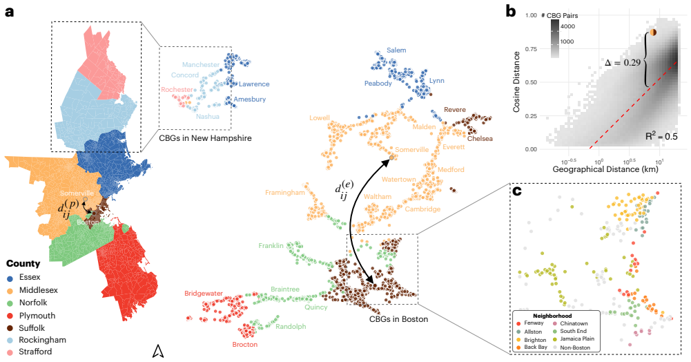
The load-bearing object is the Word2Vec skip-gram negative sampling embedding trained on trajectories: each census block group is a word, each user's sequence of visited block groups is a sentence, and the learned vector $w_i$ defines an embedding distance $d^{(e)}_{ij}=1-\frac{w_i\cdot w_j}{\|w_i\|\|w_j\|}$ that reflects how often places appear in similar movement contexts. The equivalence between this model and the gravity law of mobility justifies treating this cosine distance as a behavioral distance. A barrier is then defined operationally as a block-group pair within 20 km whose embedding distance sits in the top 5% of positive residuals from the log-linear fit $\hat{d}^{(e)}_{ij}\sim\beta\log d^{(p)}_{ij}+\varepsilon$ within each 1 km distance bin; logistic regressions with standardized predictors compare the contribution of amenity, physical, demographic, and administrative variables to the odds that a pair is a barrier.
What would settle it
Re-run the barrier detection with road-network travel time added alongside geographic distance in the residual model for any one metro, for example Boston. If the positive residuals that define the top-5% barrier pairs shrink to near zero or no longer correlate with county boundaries and income and racial distance, then the 'invisible barriers' are unmeasured physical friction and the central claim fails.
Extended reading notes
Core claim
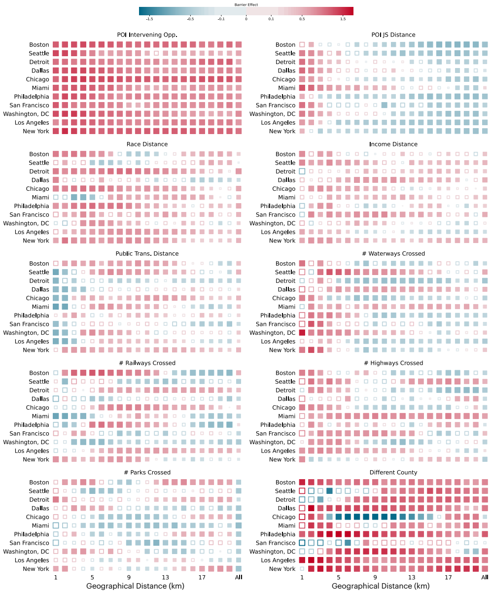
On the paper's own terms, the central discovery is that urban mobility barriers—pairs of census block groups less than 20 km apart whose embedding distance is in the top 5% of positive residuals from a log-linear fit on geographic distance—are best explained by amenity structure, administrative borders, and demographic distance. Differences in intervening opportunities, especially shopping, college, and sports venues, raise the odds of a barrier, while functional complementarity between areas lowers them; county boundaries and income and racial gaps are consistently strong predictors, and physical infrastructure is secondary and distance-dependent, with highways and parks acting as local obstacles that can facilitate movement at longer ranges. The detected barriers are concentrated in urban cores and persist across cities, spatial scales, and time periods, indicating stable behavioral structures rather than temporary artifacts.
Load-bearing premise
The whole analysis depends on the operational definition of a barrier as the top 5% of embedding residuals after a log-linear fit on geographic distance; if those residuals mostly reflect noise or unmeasured physical travel time rather than experienced disconnection, the ranking of factors that follows would be an artifact of the method.
Editorial extensions
If this is right
- Urban accessibility is primarily a product of amenity arrangement and jurisdictional and demographic divides, so maps of physical obstacles alone will mislead planning decisions.
- Changing where amenities sit can either reinforce or reduce barriers, since intervening opportunities such as shopping and college venues suppress direct movement while complementary venues, groceries, services, and transport hubs encourage it.
- Physical infrastructure has a dual role: highways, parks, railways, and waterways constrain movement at short distances but can connect places at longer distances, so barrier effects cannot be summarized by a single sign.
- The barrier structure is stable across 2019–2021 and across the 11 metros, with only a temporary pandemic shift in 2020, so the detected invisible divides reflect persistent urban structure.
- Barrier crossing is tied to discretionary and exploratory trips, and individuals from more racially diverse, transit-using, and employed neighborhoods cross barriers more often, implying that connectivity itself is unequally distributed.
Reading between the lines
- A direct testable extension the authors do not run: replace geographic distance with road-network travel time in the residual fit; if the top-5% barrier pairs largely disappear, the 'invisible' effects would be visible travel-time friction in disguise.
- The correlational design leaves causality open in both directions—diverse transit-rich neighborhoods may produce crossers, or people who cross anyway may sort into those neighborhoods—so panel or natural-experiment data would be needed to separate the two.
- Because all distances and flows are symmetric here, an editorial next step would be to use directional embeddings and ask whether barriers are asymmetric, for instance blocking low-amenity to high-amenity trips more than the reverse.
- The same embedding-residual machinery could be applied to other service geographies, such as schools or hospitals, to audit whether administrative catchment boundaries create invisible access barriers in domains beyond daily mobility.
Signed reviews
Editorial analysis
A structured set of objections, weighed in public.
Referee Report
Summary. The manuscript applies Word2Vec to CBG-level mobility trajectories from 25.4 million devices in 11 U.S. CBSAs, defining a 'mobility barrier' as a CBG pair within 20 km whose embedding cosine distance lies in the top 5% of positive residuals from a log-linear regression on geographic distance, within 1-km bins. It then fits logistic regressions of this barrier label on POI intervening opportunities, POI category complementarity, counts of crossed physical infrastructure, demographic distances, and county-boundary indicators, and reports a stable ranking across cities, years, distances, and robustness checks: amenity structure is the strongest predictor, administrative borders second, demographic segregation third, and physical infrastructure weakest. A second analysis characterizes barrier-crossing trips by time of day, venue category, and residential demographics. The paper claims that invisible, amenity- and segregation-driven barriers structure urban accessibility more than visible physical obstacles.
Significance. If the central claim survives validation, the paper is significant: it offers a scalable, data-driven way to identify behavioral disconnection between nearby neighborhoods, challenges infrastructure-centric barrier studies, and provides planning-relevant evidence on amenity layout and jurisdictional divides. Strengths include the scale (11 CBSAs, three years, 25.4 million devices), the systematic robustness checks across cities, years, spatial resolutions (H3), and pruning thresholds, the explicit link between window-1 skip-gram negative sampling and the gravity model, and public code for reproducing figures from aggregated data. The main caveat is that the barrier label is an internal residual of the embedding model and is not validated against independent measures; the stress-test concern about circularity is therefore central rather than peripheral.
major comments (3)
- [Methods, Defining Mobility Barriers; SI Note 3] The outcome variable in Eq. (1) is constructed from the top 5% residuals of an embedding distance model trained on the same trajectories whose barriers the paper aims to explain, and SI Note 3 states that most of these pairs have zero observed flow. The R^2 validation in Fig. 1c-d demonstrates that embeddings track average flows, but it does not validate the residual tails used as labels. Because Word2Vec with window=1 and min_count=50 (SI Note 4.1) gives poorly constrained vectors for low-frequency CBGs, and low-frequency CBGs may be systematically different in income, transit use, or county membership, the demographic and administrative coefficients in Eq. (1) could be artifacts of embedding frequency rather than behavioral isolation. Please add a baseline that labels barriers from residuals of observed flow, or from an independent source such as surveys or travel diaries, and rerun the full predictor ranking; also test explicitly how the ranking changes when low-frequency CBGs are excluded.
- [SI Note 3; Methods, Defining Mobility Barriers] The individual-level analysis changes the definition of the outcome: because main barrier pairs are mostly zero-flow dyads, the cross-barrier ratio is computed on 'soft barriers' defined as the top quartile of residuals among non-zero-flow pairs. The paper does not show that these soft barriers correspond to the same places or the same socioeconomic patterns as the hard barriers in Eq. (1), so Fig. 4 may characterize a different phenomenon. Please report overlap statistics between the two barrier sets and repeat the temporal and demographic analyses on the hard-barrier definition where data permit.
- [Methods, Defining Mobility Barriers; SI Section 5] The barrier definition depends on several free parameters—the 20 km cutoff, the 1 km bin size, and the top 5% residual threshold—but the robustness section varies only the flow-pruning quantiles and the spatial unit. Since the paper's headline is a ranking of predictor groups, a sensitivity analysis that varies the residual quantile (for example, top 1% and top 10%) and the distance cutoff is necessary to show that the ranking is not an artifact of one threshold choice.
minor comments (5)
- [Introduction] The sentence beginning 'To address this gap by combining large-scale mobility data...' lacks a main verb; it should read 'We address this gap by combining...'.
- [SI Note 5.1, Fig. 14] The caption of Fig. 14(b) labels the second pruning range as [0.94,0.997], while the text specifies [0.95,0.997]; these should be reconciled.
- [Abstract] The abstract contains a line-break artifact 'Y et' that should read 'Yet'.
- [SI Note 1.4; Fig. 3c] The paper would benefit from a table defining the 20 POI categories in the main text, since the taxonomy is only described in the supplementary information and is used for the headline POI effect.
- [Fig. 3b] The right-hand axis of Fig. 3b shows '50%' and '100%' ticks without explanation; please state what the normalized likelihood-ratio values represent.
Circularity Check
The headline barrier-importance ranking largely restates Stouffer's intervening-opportunities law, but the analysis contains independent external predictors and the embedding is validated against flows.
-
renaming known result
[Results, 'Identification and Nature of Mobility Barriers' (Fig. 3c); Methods, 'Defining Mobility Barriers']
"we identify CBG pairs where observed mobility is significantly lower than expected given their geographic distance... the number of intervening opportunities between CBGs is positively associated with barrier formation, as nearby alternative destinations reduce the likelihood of direct movement"
The barrier label is a high positive residual of embedding cosine distance regressed on geographic distance. Because the embeddings are trained on the same origin-destination trajectories, this residual is effectively a nonlinear proxy for abnormally low inter-CBG flow. The top-ranked predictor, POI Intervening Opportunities, is exactly Stouffer's classic mechanism for low mobility, which the paper itself states in SI Note 2.1: 'the number of persons going a given distance is ...
full rationale
No direct self-definitional circularity is present: the barrier residual is not algebraically equal to any predictor, and the main regressors (county boundaries, income/race distances, physical crossings) are measured externally from trajectories. The embedding step is independently supported within the paper by the gravity-model comparison (R2 = 0.61 vs. 0.33 in Boston, Fig. 1c-d), so the self-citation to Murray et al. for the SGNS-gravity equivalence is not load-bearing. The main circularity concern is narrower: the outcome is a flow-deficit residual, and the dominant predictor, POI intervening opportunities, is the classic Stouffer explanation for flow deficits. Thus the central 'amenity structure is primary' result is partly a re-expression of a known law in embedding coordinates. Other findings, such as the secondary role of physical infrastructure and the cross-barrier temporal/demographic patterns, are not forced by this construction and give the paper genuine independent content. Overall score reflects partial, not total, circularity.
Assumptions & free parameters
free parameters (5)
- Barrier residual threshold =
top 5% per 1 km bin
- Soft barrier threshold (cross-barrier ratio) =
top 25% among nonzero-flow pairs
- Flow pruning quantile range =
[0.95, 0.995]
- Distance cutoff and bin size =
20 km, 1 km bins
- POI attribution distance =
100 m
assumptions (4)
- domain assumption Word2Vec skip-gram with negative sampling and window size 1 is formally equivalent to the mobility gravity model.
- ad hoc to paper Large positive residuals from a log-linear fit of embedding distance on geographic distance denote real mobility barriers.
- domain assumption The Spectus opt-in smartphone panel adequately represents urban population mobility.
- domain assumption CBG-level aggregation preserves barrier-relevant movement structure.
invented entities (1)
-
Mobility barrier
Cite this review
Pith. "Pith review of Beyond Distance: Mobility Neural Embeddings Reveal Visible and Invisible Barriers in Urban Space." pith.science (2026). https://pith.science/paper/H6QUSK6S
@misc{pith2026250624061,
  author       = {Pith},
  title        = {Pith review of: Beyond Distance: Mobility Neural Embeddings Reveal Visible and Invisible Barriers in Urban Space},
  year         = {2026},
  howpublished = {\url{https://pith.science/paper/H6QUSK6S}},
  note         = {Machine review of arXiv:2506.24061}
}
read the original abstract
Human mobility in cities is shaped not only by visible structures such as highways, rivers, and parks but also by invisible barriers rooted in socioeconomic segregation, uneven access to amenities, and administrative divisions. Yet identifying and quantifying these barriers at scale and their relative importance on people's movements remains a major challenge. Neural embedding models, originally developed for language, offer a powerful way to capture the complexity of human mobility from large-scale data. Here, we apply this approach to 25.4 million observed trajectories across 11 major U.S. cities, learning mobility embeddings that reveal how people move through urban space. These mobility embeddings define a functional distance between places, one that reflects behavioral rather than physical proximity, and allow us to detect barriers between neighborhoods that are geographically close but behaviorally disconnected. We find that the strongest predictors of these barriers are differences in access to amenities, administrative borders, and residential segregation by income and race. These invisible borders are concentrated in urban cores and persist across cities, spatial scales, and time periods. Physical infrastructure, such as highways and parks, plays a secondary but still significant role, especially at short distances. We also find that individuals who cross barriers tend to do so outside of traditional commuting hours and are more likely to live in areas with greater racial diversity, and higher transit use or income. Together, these findings reveal how spatial, social, and behavioral forces structure urban accessibility and provide a scalable framework to detect and monitor barriers in cities, with applications in planning, policy evaluation, and equity analysis.
Figures


Figures from the paper (16 more)



Reference graph
Works this paper leans on
-
[1]
Mobility patterns are associated with experienced income segregation in large us cities
Esteban Moro, Dan Calacci, Xiaowen Dong, and Alex Pentland. Mobility patterns are associated with experienced income segregation in large us cities. Nature communications, 12(1):4633, 2021
work page 2021
-
[2]
Distributed representations of words and phrases and their compositionality
Tomas Mikolov, Ilya Sutskever, Kai Chen, Greg S Corrado, and Jeff Dean. Distributed representations of words and phrases and their compositionality. Advances in neural information processing systems, 26, 2013
work page 2013
-
[3]
Efficient estimation of word representations in vector space
Tomas Mikolov. Efficient estimation of word representations in vector space. arXiv preprint arXiv:1301.3781, 2013
arXiv 2013
-
[4]
Constraining weighted word co-occurrence frequencies in word embeddings
Paula Lauren. Constraining weighted word co-occurrence frequencies in word embeddings. In 2021 IEEE International Conference on Big Data (Big Data), pages 5193–5198. IEEE, 2021
work page 2021
-
[5]
American Community Survey 5-Year Data
United States Census Bureau. American Community Survey 5-Year Data. https://www.census.gov/ programs-surveys/acs, 2022. Accessed: 2024-08-22
work page 2022
-
[6]
Foursquare open source places: A new foundational dataset for the geospatial community. https://docs. foursquare.com/data-products/docs/fsq-os-places-release-notes , 2024. Accessed: 2024-11- 01
work page 2024
-
[7]
Inferring human mobility from sparse low accuracy mobile sensing data
Andrea Cuttone, Sune Lehmann, and Jakob Eg Larsen. Inferring human mobility from sparse low accuracy mobile sensing data. In Proceedings of the 2014 ACM International Joint Conference on Pervasive and Ubiquitous Computing: Adjunct Publication, pages 995–1004, 2014
work page 2014
-
[8]
Planet dump retrieved from https://planet.osm.org
OpenStreetMap contributors. Planet dump retrieved from https://planet.osm.org . https://www.openstreetmap. org, 2017
work page 2017
Show all 29 references
-
[9]
Modeling and analyzing urban networks and amenities with osmnx
Geoff Boeing. Modeling and analyzing urban networks and amenities with osmnx. Geographical Analysis, 2025
2025
-
[10]
Census Bureau
U.S. Census Bureau. TIGER Data Products Guide. https://www.census.gov/programs-surveys/ geography/guidance/tiger-data-products-guide.html , 2019. Accessed: 2024-8-22
2019
-
[11]
Intervening opportunities: a theory relating mobility and distance
Samuel A Stouffer. Intervening opportunities: a theory relating mobility and distance. American sociological review, 5(6):845–867, 1940
1940
-
[12]
Quantifying barriers of urban mobility
Gerg˝o Pintér and Balázs Lengyel. Quantifying barriers of urban mobility. arXiv preprint arXiv:2312.11343, 2023
2023 arXiv
-
[13]
Urban highways are barriers to social ties
Luca Maria Aiello, Anastassia Vybornova, Sándor Juhász, Michael Szell, and Eszter Bokányi. Urban highways are barriers to social ties. Proceedings of the National Academy of Sciences, 122(10):e2408937122, 2025
2025
-
[14]
The death and life of great American cities
Jane Jacobs. The death and life of great American cities. Modern Library, New York, 1993
1993
-
[15]
Software Framework for Topic Modelling with Large Corpora
Radim ˇReh˚ uˇrek and Petr Sojka. Software Framework for Topic Modelling with Large Corpora. In Proceedings of the LREC 2010 Workshop on New Challenges for NLP Frameworks, pages 45–50, Valletta, Malta, May 2010. ELRA. http://is.muni.cz/publication/884893/en
2010
-
[16]
Unsupervised embedding of trajectories captures the latent structure of scientific migration
Dakota Murray, Jisung Yoon, Sadamori Kojaku, Rodrigo Costas, Woo-Sung Jung, Staša Milojevi´c, and Yong-Yeol Ahn. Unsupervised embedding of trajectories captures the latent structure of scientific migration. Proceedings of the National Academy of Sciences, 120(52):e2305414120, 2023
2023
-
[17]
Principled approach to the selection of the embedding dimension of networks
Weiwei Gu, Aditya Tandon, Yong-Yeol Ahn, and Filippo Radicchi. Principled approach to the selection of the embedding dimension of networks. Nature Communications, 12(1):3772, 2021
2021
-
[18]
H3: Uber’s Hexagonal Hierarchical Spatial Index
Uber Technologies, Inc. H3: Uber’s Hexagonal Hierarchical Spatial Index. Uber Engineering Blog, June 2018
2018
-
[19]
UMAP: Uniform Manifold Approximation and Projection
Leland McInnes, John Healy, Nathaniel Saul, and Lukas Großberger. UMAP: Uniform Manifold Approximation and Projection. Journal of Open Source Software, 3(29):861, 2018
2018
-
[20]
Data Structures for Statistical Computing in Python
Wes McKinney. Data Structures for Statistical Computing in Python. In Stéfan van der Walt and Jarrod Millman, editors, Proceedings of the 9th Python in Science Conference, pages 56 – 61, 2010
2010
-
[21]
Geopandas: Python tools for geographic data, 2014
K Jordahl. Geopandas: Python tools for geographic data, 2014
2014
-
[22]
statsmodels: Econometric and statistical modeling with python
Skipper Seabold and Josef Perktold. statsmodels: Econometric and statistical modeling with python. In 9th Python in Science Conference, 2010
2010
-
[23]
Oliphant, Matt Haberland, Tyler Reddy, David Cournapeau, Evgeni Burovski, Pearu Peterson, Warren Weckesser, Jonathan Bright, Stéfan J
Pauli Virtanen, Ralf Gommers, Travis E. Oliphant, Matt Haberland, Tyler Reddy, David Cournapeau, Evgeni Burovski, Pearu Peterson, Warren Weckesser, Jonathan Bright, Stéfan J. van der Walt, Matthew Brett, Joshua Wilson, K. Jarrod Millman, Nikolay Mayorov, Andrew R. J. Nelson, E...
2020
-
[24]
John D. Hunter. Matplotlib: A 2D Graphics Environment. Computing in Science & Engineering, 9(3):90–95, 2007
2007
-
[25]
Michael L. Waskom. seaborn: statistical data visualization. Journal of Open Source Software, 6(60):3021, 2021
2021
-
[26]
ggplot2: Elegant Graphics for Data Analysis
Hadley Wickham. ggplot2: Elegant Graphics for Data Analysis. Springer-Verlag New York, 2016
2016
-
[27]
Efficient estimation of maximum likelihood models with multiple fixed-effects: the R package FENmlm
Laurent Bergé. Efficient estimation of maximum likelihood models with multiple fixed-effects: the R package FENmlm. Technical Report 2013-13, CREA Discussion Papers, 2018
2013
-
[28]
tidycensus: Load US Census Boundary and Attribute Data as ’tidyverse’ and ’sf’-Ready Data Frames, 2025
Kyle Walker and Matt Herman. tidycensus: Load US Census Boundary and Attribute Data as ’tidyverse’ and ’sf’-Ready Data Frames, 2025. R package version 1.7.1
2025
-
[29]
tigris: Load Census TIGER/Line Shapefiles, 2025
Kyle Walker. tigris: Load Census TIGER/Line Shapefiles, 2025. R package version 2.2.1. 33/40 Table 6. Estimated coefficients of model given by Eq. (1) for the 2019 study period with respective standard errors in parentheses. P-values correspond to two-sided tests for the hypot...
2025
Reviewed August 6, 2026 · model on record in the stance chip above.
Discussion (0). Continue with ORCID to comment.