REVIEW 4 major objections 5 minor 1 cited by
Learning Structured Population Models from Data with WSINDy
T0 review · 4 major / 5 minor · reviewed 2026-08-06 · deepseek-v4-flash
Pith's one-line read Adding a total-population ODE lets WSINDy recover birth, death, and growth terms of structured population models from noisy binned data.
desk verdict Solid extension of WSINDy to structured population models, but the boundary-learning claim is stronger than the math supports: β is only identified up to its projection onto the observed density. read the letter →
The pith
A machine-rendered reading of the paper's core claim, the machinery that carries it, and where it could break.
The reading
What carries the argument
The load-bearing object is the stacked weak-form linear system $b = Gw$ of Equation (9). The PDE block is assembled from inner products of compactly supported piecewise-polynomial test functions with transport and source library terms, while the ODE block is assembled from the weak form of $dN/dt = \int \beta n + \int f$, with the total population $N$ computed from the same binned data. Sparse weights $w = (w_g, w_f, w_\beta)$ are found by minimizing $\|b - Gw\|^2 + \lambda\|w\|_0$ with modified sequential thresholding least squares. Because the PDE block has far more rows, the boundary-bagging step fixes $w_f$ and refits $w_\beta$ from the ODE residual, then prunes the boundary library to the support intersection (or union) of the two fits before refitting. This combination moves boundary information into the regression and keeps the sparse solution from pushing all error into the birth term.
What would settle it
Simulate a structured population model whose true birth rate is a Gaussian with mean lying between two library Gaussians, add low-level log-normal noise, and run the algorithm; because the true term is absent from the library, exact recovery is impossible and the returned coefficients will be systematically biased, demonstrating that the central recovery claim is conditional on the library containing the true ingredients.
Extended reading notes
Core claim
The paper claims that the true transport, source, and boundary ingredients of a structured population model can be recovered simultaneously from noisy histogram data by solving one stacked sparse linear system. The interior weak form of the hyperbolic PDE yields rows that constrain the growth term and the mortality term, but the compactly supported test functions erase the birth process at the inflow boundary. The paper therefore adds the weak form of the total-population ODE obtained by integrating the PDE over the whole structural domain, whose rows carry the boundary information through the birth kernel and the source term. Concatenating the two blocks and applying modified sequential thresholding least squares, with the boundary-bagging step to counter the imbalance between the large PDE block and the small ODE block, returns sparse coefficient vectors that select the correct library terms; in the synthetic tests the method recovers the true coefficients at low noise, and in misspecified libraries it can still return effective models with low prediction error.
Load-bearing premise
The true growth, death, and birth functions must be exactly sparse linear combinations of the user-supplied library trial functions, and any nonlinear parameters in those functions must be fixed in advance.
Editorial extensions
If this is right
- With a library that contains the true model ingredients, the stacked system recovers transport, source, and boundary coefficients from noisy histogram data without forward simulation; the paper reports per-realization run times under ten seconds on a laptop.
- If the true ingredients are not in the library, the learned model can still predict the population well even when its term support is wrong, so the output is best interpreted as an effective hypothesis over the supplied library rather than the true mechanism.
- Library distinguishability is a practical bottleneck: as candidate functions are spaced closer together, the condition number of the weak-form matrix grows and the true-positive ratio drops sharply, so nearly redundant trial functions should be excluded.
- For density-dependent models, data that converge quickly to equilibrium make different functions of total population $N$ look alike, and the algorithm may substitute a sparser linear or lower-order approximation; this is a documented limitation rather than a resolved issue.
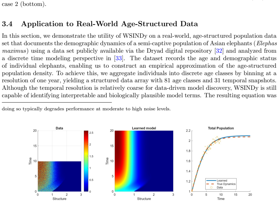
- When the aging rate is known a priori for age-structured data, moving that transport term into the data vector focuses the regression entirely on death and birth, which is how the elephant-data application is handled.
Reading between the lines
- A direct extension suggested by the paper's own discussion would close the loop between library construction and selection: after a first regression selects a family, re-estimate that family's nonlinear parameters and re-run the selection until the active matrix's condition number drops.
- The boundary-bagging trick is a general recipe for weak-form discovery: when compactly supported test functions erase a process, append an aggregated conservation equation for that process and arbitrate the two fits by support intersection; the same construction should apply to conservation laws, moment systems, and flux boundary conditions beyond population biology.
- The distinguishability experiments imply a testable screening rule: success rate on a given library and dataset should track the condition number of the weak-form matrix, so candidate libraries could be rejected a priori when that condition number exceeds a threshold, before any regression is run.
Editorial analysis
A structured set of objections, weighed in public.
Referee Report
Summary. The manuscript extends the Weak SINDy (WSINDy) framework to structured population models of the form (3). Given noisy histogram observations of the population density n(t,s), the method builds a weak-form linear system from an interior PDE test-function equation (4), stacks it with a weak form of the total-population ODE (7), and uses sparse regression to select transport, source, and boundary terms from a user-supplied library. A 'boundary bagging' heuristic (Algorithm 1) refits the boundary coefficients from the ODE residual. The method is tested on four linear and two nonlinear synthetic examples under multiplicative lognormal noise, on a library-distinguishability study, and on an Asian elephant age-structured dataset, with metrics including coefficient errors, true positivity ratio, and temporal holdout prediction error.
Significance. If the claims are substantiated, the method would provide a fast, interpretable alternative to repeated forward-solve parameter estimation for structured population models, and the temporal holdout prediction error provides an out-of-sample check that strengthens the empirical case. The authors are appropriately explicit about limitations such as library exactness, test-function hyperparameters, and the distinguishability of similar library terms. The code release and the real-data comparison to an established matrix model are also useful contributions. However, the central claim that the boundary process is learned 'directly from the data' is currently stronger than the information content of the stacked system supports, and the synthetic experiments do not isolate that failure mode.
major comments (4)
- [Section 2.2, Eqs. (6)-(9)] The boundary term β* appears in the stacked system only through the scalar integral ∫_Ω β(s)n(t,s) ds in Eq. (7), while the PDE weak form (4) uses test functions compactly supported in the interior of Ω and therefore contains no boundary information. Consequently, the stacked system can identify β only up to its projection onto the span of the observed densities n(t,·) over the sampled times; two library functions that produce nearly identical values of this integral at the sampled times cannot be distinguished by any regression on Eq. (9). The manuscript does not state or verify identifiability conditions (e.g., sufficient variation of n(t,s) in s and t, or boundary-local test functions), and the aggregate TPR/E2 metrics in Section 3.2 do not isolate the boundary component. This gap is load-bearing for the abstract's claim of learning the boundary process directly from the data.
- [Section 2.2.1, Algorithm 1] The proposed 'boundary bagging' procedure is not a cross-validation method: it uses the same ODE rows and the already-fitted source weights to refit β from the residual b_ode − Ξ_f w_f, with no held-out data. It therefore cannot create information about β that is absent from Eq. (7). Calling it cross-validation in the abstract and in Section 2.2.1 overstates what the procedure does. The support-intersection heuristic may be a reasonable stability check, but the manuscript should either describe it as such or compare it with an actual data-splitting scheme.
- [Section 3.2.2 and Figure 3] The distinguishability experiments fix the transport and the non-target component to the true terms and vary only the spacing of candidate functions; they report TPR and condition numbers, but they do not quantify how much information about the boundary term is present in the observed density snapshots. As a result, the experiments do not resolve the projection-identifiability issue raised by Eq. (7). Please add either an information-theoretic or coherence analysis of the stacked system, or a demonstration with intentionally information-poor data (e.g., densities that quickly converge to a stable shape) showing when boundary recovery succeeds and fails.
- [Section 4, Discussion versus Figure 1] The Discussion states that WSciML methods are 'highly robust to noise' and cites Figure 1, but Figure 1 shows the true positivity ratio dropping from 1 to roughly 0.6-0.8 as σNR increases, with prediction error remaining low. This is not necessarily a contradiction, but the robustness claim should be qualified to mean robust predictive performance rather than robust term selection; otherwise the text promises stronger support than the reported metrics provide.
minor comments (5)
- [Section 3.2.1 and Figure 2] The text says the TPR = 0.8 example is problem L.2, while the Figure 2 caption says example L.3; please reconcile this inconsistency.
- [Section 1 and Section 4] Section 1 contains the duplicated phrase 'the the Weak-form Estimation'; Section 4 also repeats the sentence 'It is of course, still necessary to carefully curate a library...' verbatim in consecutive paragraphs.
- [Figure 8 caption] The caption uses 'respectfully' where 'respectively' is meant.
- [Section 3.1] The statement that nonlinear parameters must be given in the library is important and should appear earlier, perhaps in the abstract or introduction, since it defines the scope of 'selection' and directly affects the practical applicability of the method.
- [Table 3] The boundary library notation for L.2 uses {f_Gauss(s; 5k, 5)}_{k=1,2,3}; the later text refers to f_Gauss(s; 10, 5) as the true term in Case 2, which matches k=2, but the notation is easy to misread and should be clarified.
Circularity Check
No significant circularity: the stacked weak-form system is a regression fit to data, and the prediction error is evaluated on an out-of-sample time interval; self-citations are provenance, not load-bearing assumptions.
full rationale
The paper's derivation chain is self-contained as a data-fitting and model-selection method. Equation (4) is the standard weak form of the interior PDE, and because the compactly supported test functions omit the boundary condition, the authors introduce the total-population ODE (6) obtained by integrating (3), with weak form (7). Stacking the interior PDE system (5) with the ODE system (8) gives the full regression problem (9). The coefficients w are fit to the observed histogram data via sparse regression, and the reported prediction error Ep is defined by simulating the learned model over the holdout interval (Ttest, T) and comparing to the true solution; it is not the training residual, so the prediction is not a disguised fit. The boundary-bagging refinement in Algorithm 1 refits only the boundary weights from the ODE residual bode - Ξf wf; this is a model-selection heuristic and does not make the learned boundary process an input to itself. The paper also explicitly acknowledges the distinguishability and identifiability limitations of the boundary term, noting that the ODE rows contain only the averaged quantity integral of beta times n, so this is an identifiability caveat rather than a circular construction. Citations to prior WSINDy work by the same group provide the algorithmic foundation of MSTLS and weak-form integration, but the present extension, including heterogeneous dynamics and boundary-process learning, is derived from the model equations and evaluated on independent synthetic and real data. No equation in the paper is defined in terms of a fitted output, no fitted parameter is renamed as a prediction, and no load-bearing argument reduces to a self-citation. Therefore the appropriate circularity score is 0.
Assumptions & free parameters
free parameters (5)
- Test function support radii r_s and r_t =
0.5
- Test function polynomial order p = q =
14
- Sparsity threshold / lambda in loss function =
not specified
- Real-data library shape parameters =
Gaussian fertility mean=33, sd=11; mortality rate 0.06, shift 85
- Loess smoothing parameters for variance estimation =
not specified
assumptions (5)
- domain assumption Data are generated by a hyperbolic structured population PDE of the form (3) with smooth or globally Lipschitz coefficients.
- domain assumption True model ingredients are sparse linear combinations of the trial functions in the user-selected library.
- standard math Trapezoidal rule convergence lemma from Messenger and Bortz [14] applies to the weak-form integrals with the chosen test functions.
- domain assumption The total population ODE (Eq. 6) is exact for the data, i.e., the boundary conditions (3b)-(3c) hold in aggregate.
- domain assumption Multiplicative lognormal noise model and the bias correction using loess-estimated variance.
Cite this review
Pith. "Pith review of Learning Structured Population Models from Data with WSINDy." pith.science (2026). https://pith.science/paper/QK3QWNTW
@misc{pith2026250624101,
  author       = {Pith},
  title        = {Pith review of: Learning Structured Population Models from Data with WSINDy},
  year         = {2026},
  howpublished = {\url{https://pith.science/paper/QK3QWNTW}},
  note         = {Machine review of arXiv:2506.24101}
}
read the original abstract
In the context of population dynamics, identifying effective model features, such as fecundity and mortality rates, is generally a complex and computationally intensive process, especially when the dynamics are heterogeneous across the population. In this work, we propose a Weak form Scientific Machine Learning-based method for selecting appropriate model ingredients from a library of scientifically feasible functions used to model structured populations. This method uses extensions of the Weak form Sparse Identification of Nonlinear Dynamics (WSINDy) method to select the best-fitting ingredients from noisy time-series histogram data. This extension includes learning heterogeneous dynamics and also learning the boundary process of the model directly from the data. We additionally provide a cross-validation method which helps fine tune the recovered boundary process to the data. Several test cases are considered, demonstrating the method's performance for different previously studied models, including age and size-structured models. Through these examples, we examine both the advantages and limitations of the method, with a particular focus on the distinguishability of terms in the library.
Figures


Figures from the paper (5 more)


Forward citations
Cited by 1 Pith paper
-
Weak Form Scientific Machine Learning: Test Function Construction for System Identification
A new algorithm picks the support radius of weak-form test functions by locating the changepoint of an estimated integration error curve, and this radius lands near the parameter-error minimum in most tested cases.
Reference graph
Works this paper leans on
-
[1]
J. A. J. Metz, O. Diekmann, and S. Levin, eds., The Dynamics of Physiologically Structured Populations, vol. 68 of Lecture Notes in Biomathematics . Berlin, Heidelberg: Springer Berlin Heidelberg, 1986
work page 1986
-
[2]
Some Remarks on Changing Populations,
H. Von Foerster, “Some Remarks on Changing Populations,” in The Kinetics of Cellular Prolif- eration (F. Stohlman, ed.), pp. 382–407, Grune & Stratton, 1959
work page 1959
-
[3]
The McKendrick partial differential equation and its uses in epi- demiology and population study,
B. Keyfitz and N. Keyfitz, “The McKendrick partial differential equation and its uses in epi- demiology and population study,” Mathematical and Computer Modelling , vol. 26, pp. 1–9, Sept. 1997
work page 1997
-
[4]
Applications of Mathematics to Medical Problems,
A. G. McKendrick, “Applications of Mathematics to Medical Problems,” Proc. Edinb. Math. Soc., vol. 44, p. 98, Feb. 1925
work page 1925
-
[5]
A New Model For Age-Size Structure of a Population,
J. W. Sinko and W. Streifer, “A New Model For Age-Size Structure of a Population,” Ecology, vol. 48, pp. 910–918, Nov. 1967
work page 1967
-
[6]
Rapidly converging numerical algorithms for models of population dynamics,
F. A. Milner and G. Rabbiolo, “Rapidly converging numerical algorithms for models of population dynamics,” J. Math. Biol. , vol. 30, Aug. 1992
work page 1992
-
[7]
Determining a Coefficient in a First-Order Hyperbolic Equation,
M. Pilant and W. Rundell, “Determining a Coefficient in a First-Order Hyperbolic Equation,” SIAM J. Appl. Math. , vol. 51, pp. 494–506, Apr. 1991
work page 1991
-
[8]
Non-linear age-dependent population dynamics,
M. E. Gurtin and R. C. Maccamy, “Non-linear age-dependent population dynamics,” Arch. Ra- tional Mech. Anal. , vol. 54, pp. 281–300, Sept. 1974
work page 1974
Show all 42 references
-
[9]
Some competition models for size-structured populations,
J. Cushing, “Some competition models for size-structured populations,” Rocky Mountain J. Math., vol. 20, Dec. 1990
1990
-
[10]
Inverse Problems and Structured-Population Dynamics,
S. N. Wood, “Inverse Problems and Structured-Population Dynamics,” in Structured-Population Models in Marine, Terrestrial, and Freshwater Systems (S. Tuljapurkar and H. Caswell, eds.), pp. 555–586, Boston, MA: Springer US, 1997
1997
-
[11]
Discovering governing equations from data by sparse identification of nonlinear dynamical systems,
S. L. Brunton, J. L. Proctor, and J. N. Kutz, “Discovering governing equations from data by sparse identification of nonlinear dynamical systems,” Proc. Natl. Acad. Sci. , vol. 113, pp. 3932–3937, Apr. 2016. 15
2016
-
[12]
Data-driven discovery of partial differential equations,
S. H. Rudy, S. L. Brunton, J. L. Proctor, and J. N. Kutz, “Data-driven discovery of partial differential equations,” Sci. Adv., vol. 3, p. e1602614, Apr. 2017
2017
-
[13]
Weak SINDy For Partial Differential Equations,
D. A. Messenger and D. M. Bortz, “Weak SINDy For Partial Differential Equations,” J. Comput. Phys., vol. 443, p. 110525, Oct. 2021
2021
-
[14]
Weak SINDy: Galerkin-Based Data-Driven Model Selection,
D. A. Messenger and D. M. Bortz, “Weak SINDy: Galerkin-Based Data-Driven Model Selection,” Multiscale Model. Simul. , vol. 19, no. 3, pp. 1474–1497, 2021
2021
-
[15]
Direct Estimation of Parameters in ODE Mod- els Using WENDy: Weak-form Estimation of Nonlinear Dynamics,
D. M. Bortz, D. A. Messenger, and V. Dukic, “Direct Estimation of Parameters in ODE Mod- els Using WENDy: Weak-form Estimation of Nonlinear Dynamics,” Bull. Math. Biol. , vol. 85, no. 110, 2023
2023
-
[16]
WENDy for Nonlinear-in- Parameter ODEs,
N. Rummel, D. A. Messenger, S. Becker, V. Dukic, and D. M. Bortz, “WENDy for Nonlinear-in- Parameter ODEs,” arXiv:2502.08881, Feb. 2025
2025
-
[17]
Weak form-based data-driven modeling: Compu- tationally Efficient and Noise Robust Equation Learning and Parameter Inference,
D. M. Bortz, D. A. Messenger, and A. Tran, “Weak form-based data-driven modeling: Compu- tationally Efficient and Noise Robust Equation Learning and Parameter Inference,” in Numerical Analysis Meets Machine Learning (S. Mishra and A. Townsend, eds.), vol. 25 of Handbook of Num...
2024
-
[18]
The Weak Form Is Stronger Than You Think,
D. A. Messenger, A. Tran, V. Dukic, and D. M. Bortz, “The Weak Form Is Stronger Than You Think,” SIAM News , vol. 57, Oct. 2024
2024
-
[19]
Measure-valued solutions for a hierarchically size-structured population,
A. S. Ackleh and K. Ito, “Measure-valued solutions for a hierarchically size-structured population,” J. Differ. Equ. , vol. 217, pp. 431–455, Oct. 2005
2005
-
[20]
A structured coagulation-fragmentation equation in the space of radon measures: Unifying discrete and continuous models,
A. S. Ackleh, R. Lyons, and N. Saintier, “A structured coagulation-fragmentation equation in the space of radon measures: Unifying discrete and continuous models,” ESAIM: M2AN, vol. 55, pp. 2473–2501, Sept. 2021
2021
-
[21]
D¨ ull, P
C. D¨ ull, P. Gwiazda, A. Marciniak-Czochra, and J. Skrzeczkowski,Spaces of Measures and Their Applications to Structured Population Models . Cambridge University Press, 2021
2021
-
[22]
The ultimate-sustainable-yield problem in nonlinear age-structured populations,
W. M. Getz, “The ultimate-sustainable-yield problem in nonlinear age-structured populations,” Mathematical Biosciences, vol. 48, pp. 279–292, Apr. 1980
1980
-
[23]
Perthame, Transport Equations in Biology
B. Perthame, Transport Equations in Biology. Frontiers in Mathematics, Basel: Birkh¨ auser Basel, 2007
2007
-
[24]
Influence of four major plant traits on average height, leaf-area cover, net primary productivity, and biomass density in single-species forests: A theoretical investigation,
D. S. Falster, ˚A. Br¨ annstr¨ om, U. Dieckmann, and M. Westoby, “Influence of four major plant traits on average height, leaf-area cover, net primary productivity, and biomass density in single-species forests: A theoretical investigation,” Journal of Ecology , vol. 99, pp. 1...
2011
-
[25]
On the dynamics of chemically stressed populations: The deduction of population consequences from effects on individuals,
S. Kooijman and J. Metz, “On the dynamics of chemically stressed populations: The deduction of population consequences from effects on individuals,” Ecotoxicology and Environmental Safety, vol. 8, pp. 254–274, June 1984
1984
-
[26]
Learning Weather Models from Data with WSINDy,
S. Minor, D. A. Messenger, V. Dukic, and D. M. Bortz, “Learning Weather Models from Data with WSINDy,” arXiv:2501.00738, Jan. 2025
2025 arXiv
-
[27]
Weak-form inference for hybrid dynamical systems in ecology,
D. A. Messenger, G. Dwyer, and V. Dukic, “Weak-form inference for hybrid dynamical systems in ecology,” J. R. Soc. Interface. , vol. 21, p. 20240376, Dec. 2024
2024
-
[28]
Ensemble-SINDy: Robust sparse model discovery in the low-data, high-noise limit, with active learning and control,
U. Fasel, J. N. Kutz, B. W. Brunton, and S. L. Brunton, “Ensemble-SINDy: Robust sparse model discovery in the low-data, high-noise limit, with active learning and control,” Proc. R. Soc. A. , vol. 478, p. 20210904, Apr. 2022
2022
-
[29]
On the heterogeneity of human populations as reflected by mortality dynamics,
D. Avraam, S. Arnold, O. Vasieva, and B. Vasiev, “On the heterogeneity of human populations as reflected by mortality dynamics,” Aging, vol. 8, pp. 3045–3064, Nov. 2016
2016
-
[30]
Pareto-based optimization of sparse dynam- ical systems,
G. Ducci, M. Kouyate, K. Reuter, and C. Scheurer, “Pareto-based optimization of sparse dynam- ical systems,” J. Chem. Phys. , vol. 162, p. 114118, Mar. 2025. 16
2025
-
[31]
Finite difference schemes for a structured population model in the space of measures,
A. S. Ackleh, R. Lyons, and N. Saintier, “Finite difference schemes for a structured population model in the space of measures,” Math. Biosci. Eng. , vol. 17, no. 1, pp. 747–775, 2020
2020
-
[32]
Data from: Changes in age-structure over four decades were a key determinant of population growth rate in a long-lived mammal,
J. Jackson, K. Mar, W. Htut, D. Childs, and V. Lummaa, “Data from: Changes in age-structure over four decades were a key determinant of population growth rate in a long-lived mammal,” July 2020
2020
-
[33]
Changes in age-structure over four decades were a key determinant of population growth rate in a long-lived mammal,
J. Jackson, K. U. Mar, W. Htut, D. Z. Childs, and V. Lummaa, “Changes in age-structure over four decades were a key determinant of population growth rate in a long-lived mammal,” Journal of Animal Ecology, vol. 89, pp. 2268–2278, Oct. 2020
2020
-
[34]
Asymptotic consistency of the WSINDy algorithm in the limit of continuum data,
D. A. Messenger and D. M. Bortz, “Asymptotic consistency of the WSINDy algorithm in the limit of continuum data,” IMA J. Numer. Anal. , p. drae086, Dec. 2024
2024
-
[35]
Influence of initial conditions on data-driven model identification and information entropy for ideal mhd problems,
G. Vasey, D. Messenger, D. Bortz, A. Christlieb, and B. O’Shea, “Influence of initial conditions on data-driven model identification and information entropy for ideal mhd problems,” Journal of Computational Physics , vol. 524, p. 113719, Mar. 2025
2025
-
[36]
DoE-integrated Sparse Identification of Nonlinear Dynamics for Au- tomated Model Generation and Parameter Estimation in Kinetic Studies,
W. Lyu and F. Galvanin, “DoE-integrated Sparse Identification of Nonlinear Dynamics for Au- tomated Model Generation and Parameter Estimation in Kinetic Studies,” in Computer Aided Chemical Engineering, vol. 53, pp. 169–174, Elsevier, 2024
2024
-
[37]
Estimation of growth and survival in size-structured cohort data: An application to larval striped bass (Morone saxatilis),
H. T. Banks, L. W. Botsford, F. Kappel, and C. Wang, “Estimation of growth and survival in size-structured cohort data: An application to larval striped bass (Morone saxatilis),” J. Math. Biol., vol. 30, pp. 125–150, 1991
1991
-
[38]
Estimation of Cell Proliferation Dynamics Using CFSE Data,
H. T. Banks, K. L. Sutton, W. Clayton Thompson, G. Bocharov, D. Roose, T. Schenkel, and A. Meyerhans, “Estimation of Cell Proliferation Dynamics Using CFSE Data,” Bull. Math. Biol. , vol. 73, pp. 116–150, Jan. 2011
2011
-
[39]
Finite difference approximations for measure- valued solutions of a hierarchicallysize-structured population model,
A. S. Ackleh, V. K. Chellamuthu, and K. Ito, “Finite difference approximations for measure- valued solutions of a hierarchicallysize-structured population model,” Math. Biosci. Eng. , vol. 12, no. 2, pp. 233–258, 2015
2015
-
[40]
High resolution finite difference schemes for a size structured coagulation-fragmentation model in the space of radon measures,
A. S. Ackleh, R. Lyons, and N. Saintier, “High resolution finite difference schemes for a size structured coagulation-fragmentation model in the space of radon measures,” MBE, vol. 20, no. 7, pp. 11805–11820, 2023
2023
-
[41]
A Second-Order High-Resolution Scheme for a Juvenile-Adult Model of Amphibians,
A. S. Ackleh and B. Ma, “A Second-Order High-Resolution Scheme for a Juvenile-Adult Model of Amphibians,” Numer. Funct. Anal. Optim. , vol. 34, pp. 365–403, Apr. 2013
2013
-
[42]
F. E. Harrell, Regression Modeling Strategies: With Applications to Linear Models, Logistic and Ordinal Regression, and Survival Analysis . Springer Series in Statistics, Cham: Springer Interna- tional Publishing, 2015. A Simulation details Due to the histogram-style interpret...
2015
Reviewed August 6, 2026 · model on record in the stance chip above.
Discussion (0). Continue with ORCID to comment.