REVIEW 4 major objections 5 minor 48 references
Weak Form Scientific Machine Learning: Test Function Construction for System Identification
T0 review · 4 major / 5 minor · reviewed 2026-08-06 · deepseek-v4-flash
Pith's one-line read In weak-form system identification, the radius of the test functions that minimizes numerical integration error also minimizes parameter-estimation error, and it can be identified from noisy data alone.
desk verdict Useful heuristic with real technical content, but the central conjecture is unproved and the paper's own high-noise examples show the radius-selection claim failing. read the letter →
The pith
A machine-rendered reading of the paper's core claim, the machinery that carries it, and where it could break.
The reading
What carries the argument
The load-bearing object is the surrogate integration-error curve $\hat e(U,r)$ from Proposition 2.4, together with Conjecture 2.2 that its changepoint equals the parameter-error-minimizing radius. The estimator is built from Lemma 2.3's asymptotic expansion of the trapezoidal error, $\hat e_{\mathrm{int}}=(1/\sqrt{T})PF\hat\Psi I$, where $P$ selects rows at test-function centers, $F$ is the DFT matrix, $\hat\Psi$ is the diagonal matrix of Fourier coefficients of the reference function, and $I$ contains endpoint values and finite-difference endpoint derivatives from the Euler–Maclaurin series truncated at order $S$. For the piecewise polynomial family, Proposition 3.1 gives those Fourier coefficients in closed form through Bessel functions, so the sweep over radii is cheap. The changepoint is located by Algorithm B.1, which fits two line segments to the log curve and picks the break minimizing relative fitting error; this mechanism converts an unobservable quantity (expected parameter error) into an observable curve feature.
What would settle it
Run WENDy-OLS on logistic-growth data with high noise (e.g., 40 percent) and compare the radius selected by Algorithm 2.1 to the radius giving the smallest median parameter error over many realizations; the paper's own Figure 4 shows these already diverge there, so a single clean reproduction of that divergence under the paper's stated conditions would settle Conjecture 2.2.
Extended reading notes
Core claim
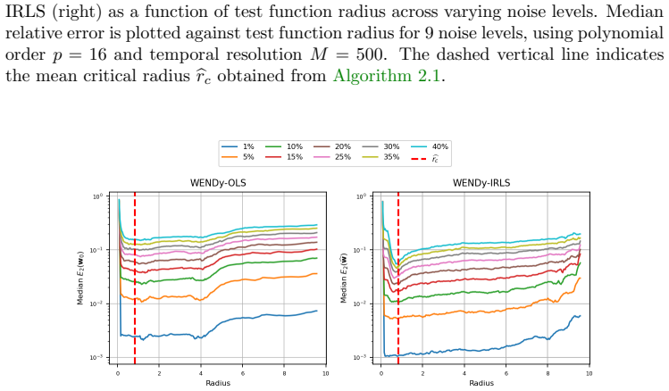
The paper's central claim is Conjecture 2.2: for the WENDy estimator with test-function radius $r$, the expected parameter error $\mathbb{E}[\|\hat w(r)-w^\star\|^2]$ is minimized at the radius $r_c$ where the monotone decrease of $\log\|e_{\mathrm{int}}(r)\|$ stagnates. The supporting discovery is that this stagnation radius can be found without knowing $w^\star$ or the clean trajectory $u^\star$: Proposition 2.4 gives an estimator $\hat e_{\mathrm{int}}$ based on a truncated Euler–Maclaurin expansion of the trapezoidal-rule error, the closed-form Fourier coefficients of the piecewise-polynomial reference function $\psi(t;r,p)=C(r-t)^p(r+t)^p$, and boundary derivatives computed by finite differences. Algorithm 2.1 sweeps $r$, applies a two-segment changepoint detector to $\log \hat e(U,r)$, and returns that radius as the construction radius. The numerical sections present this as consistently landing in low parameter-error regions, with the qualification that under WENDy-OLS the alignment degrades for strong nonlinearities at high noise.
Load-bearing premise
The method works only if the radius where the estimated integration error stops decreasing is the same radius that minimizes parameter error, and only if noisy measurements can stand in for the true trajectory in finding that radius without moving it.
Editorial extensions
If this is right
- Manual tuning of the test-function support size is no longer needed: the critical radius is computed from the data by Algorithm 2.1, requiring neither the true parameters nor noise-free data.
- Across the tested systems the selected radius aligns with low parameter error under both WENDy-OLS and WENDy-IRLS in most settings, with the strongest misalignments appearing under OLS for logistic growth and FitzHugh–Nagumo at high noise.
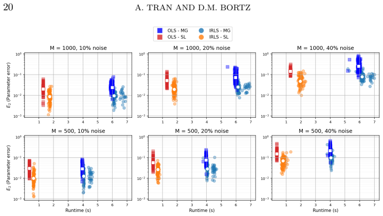
- The single-scale-local construction is consistently faster than the multiscale-global construction, with median IRLS runtime improvements of roughly 60–70 percent on several of the test systems.
- For piecewise polynomial test functions, the paper gives a practical order guideline: choosing $p$ between 16 and 22 is sufficient for the tested resolutions, with integration error scaling at least as $O(\Delta t^p)$ for even $p$.
Reading between the lines
- An unstated consequence is that the same changepoint rule could select support sizes for weak-form PDE learning and model discovery, where manual scale choice is a known practical bottleneck.
- A testable extension is to iterate the radius selection as parameter estimates improve, since the paper fixes the estimator while sweeping radii but WENDy-IRLS updates the covariance during iterations.
- The paper's own high-noise OLS results suggest the changepoint alignment depends on the regression bias being small; this predicts that the radius rule is most reliable when paired with a covariance-corrected or debiased estimator.
- Because the estimator needs only endpoint derivatives, it may transfer to non-uniform or streaming time grids, though the paper only treats uniform grids.
Editorial analysis
A structured set of objections, weighed in public.
Referee Report
Summary. The paper proposes a data-driven procedure for selecting the support radius of compactly supported test functions in weak-form parameter estimation (WENDy/WSINDy). The central idea is to approximate the numerical integration error induced by quadrature, using an Euler–Maclaurin expansion that is independent of the true parameters, and then to choose the radius where the estimated integration-error curve changes from exponential decay to stagnation. This radius is conjectured to coincide with the radius minimizing expected parameter error (Conjecture 2.2). The authors derive an asymptotic expansion of the integration error (Lemma 2.3), construct an efficient FFT-based estimator (Proposition 2.4), propose Algorithm 2.1, give practical guidance for piecewise polynomial test functions, and validate the approach on logistic growth, Duffing, Lorenz, and FitzHugh–Nagumo systems under WENDy-OLS and WENDy-IRLS, also comparing with their earlier Multi-scale-Global method.
Significance. If the central conjecture were established or its validity regime were clearly characterized, the method would give a practical answer to a long-standing hyperparameter question in weak-form scientific machine learning: how to select the test-function support from noisy data alone. The derivation of the integration-error estimator (Lemma 2.3 and Proposition 2.4) is a genuine contribution: the estimator is explicitly independent of the unknown parameters, computable via FFTs, and supported by extensive numerical experiments across several ODE systems, noise levels, and resolutions. The paper is also honest in stating that Conjecture 2.2 is unproved and left for future work. However, the paper's own numerical results contain configurations in which the selected radius does not align with the low-parameter-error region, so the advertised claim of consistent alignment is too strong. The main value of the paper is thus as a promising, well-engineered heuristic with a rigorous error-expansion foundation, rather than as a fully validated automatic selection rule.
major comments (4)
- [Section 2.2, Conjecture 2.2] Conjecture 2.2 is the load-bearing assertion of the paper: it identifies the changepoint of the monotone decrease of log(||eint(r)||) with the minimizer of expected parameter error. The assumptions stated before the conjecture are not satisfied by the WENDy-OLS problem in general. In the residual decomposition (2.1), the parameter error is driven by eTheta, r0, eint, and noise; when the regression matrix G is a nonlinear function of noisy data, the residual is not zero-mean and minimizing eint alone need not minimize E[||w_hat - w*||^2]. The paper does not provide a proof or a precise characterization of when the conjecture holds, nor does it bound the discrepancy. Since Algorithm 2.1 and the abstract's central claim rely on this conjecture, the manuscript needs either a proof under stated conditions, a quantitative bound on the deviation, or a clearly limited validity claim with supporting analysis.
- [Remark 2.9] The transition from true trajectory u* to noisy measurements U inside the error estimator is asserted without proof. The estimator be(U,S,mu) requires finite-difference approximations of derivatives up to order 2S at the endpoints. For S=1 and dt=0.02, a second-derivative finite-difference stencil amplifies noise by a factor of order 1/dt^2, which can shift the estimated changepoint relative to the true integration-error changepoint. The remark claims this is 'substantially mitigated' because only boundary points are used, but no variance or bias analysis is provided. The paper needs either a quantitative analysis of this noise-induced shift or a numerical study that explicitly tests the sensitivity of brc to the finite-difference stencil order and dt across the noise regimes used in the experiments.
- [Section 4.1, Figures 4 and 7] The paper's own results contradict the abstract's statement that selected supports 'consistently align with regions of minimal parameter estimation error'. For logistic growth under WENDy-OLS (Figure 4, left) and for FitzHugh–Nagumo under both OLS and IRLS (Figure 7), the dashed brc line falls outside the low-parameter-error region at noise ratios above roughly 5%, with the discrepancy growing with noise. The text in Section 4.1 acknowledges these cases but the abstract and Section 5 do not carry the caveat. The central claim must be reworded to state the observed validity regime, and the method should be accompanied by guidance (or a diagnostic) for detecting when the selected radius is unreliable.
- [Section 2.3 and Definition 2.6] The changepoint of the estimated error curve is computed by Algorithm B.1 on log(be(r)), but the error metric E(k) in Algorithm B.1 divides by the function values ym. For the integration-error curve, which decays to near machine precision and can cross zero or become negative in finite-precision arithmetic, the relative-error formulation can be unstable and the changepoint may depend sensitively on the lower tail of the curve. The paper does not discuss this numerical issue or justify the choice of relative error over an absolute error or a fit in log-space. A brief analysis or a robustness check (e.g., varying the changepoint algorithm's tolerance) would strengthen the reproducibility of brc.
minor comments (5)
- [Page 4, equation (1.3) context] There is a typo 'Θ(U) ∈∈ R' in the definition of the discrete feature matrix; the double '∈' should be a single symbol.
- [Page 6, Conjecture 2.2 and surrounding text] The sentence 'We choose brc (defined as the change point of be(r)) as the reference test function radius. and construct the test function set K' contains a period before 'and'; this should be corrected.
- [Section 4.2, Figure 11 reference] In the paragraph beginning 'However, the MG approach can sometimes offer runtime advantages', the reference 'Lorenz system under WENDy-IRLS(Figure 11)' should be 'Figure 13'; the Lorenz results are shown in Figure 13, not Figure 11.
- [Section 3.1, paragraph after Figure 3] The text says 'As ∆t increases, higher values of p are required' but the discussion of the scaling is for the integration error only; a sentence clarifying that this is independent of noise effects would help avoid misinterpretation.
- [Appendix I, Figure 15] The figure caption says 'for the Lorenz system (left) and logistic growth model (right)' but the main text does not describe the plotted curves beyond the legend; adding a sentence explaining the colored lines and the takeaway about fM would improve readability.
Circularity Check
No significant circularity: the radius-selection rule is derived from an independent integration-error expansion and tested against true parameter error, not fitted to it.
full rationale
The paper's central chain is not circular. Lemma 2.3 expands the trapezoidal integration error eint(phi,u*) via the Euler-Maclaurin formula in terms of endpoint values and derivatives of u*, with no dependence on the unknown parameters w*. Proposition 2.4 turns this into an estimator beint(U,S,mu) computed only from data, and Algorithm 2.1 selects the changepoint of log(be(U,r)) as the critical radius. The link between this changepoint and minimal parameter error is explicitly stated as Conjecture 2.2, an unproved assumption rather than a definitional identity or a fitted relation; the paper acknowledges "a rigorous mathematical or statistical justification remains open." The numerical sections compare the selected brc with median parameter error computed using the true w*, so the agreement is an empirical validation, not a fitted quantity renamed as a prediction. Prior work by the same authors ([3], [23], [24]) is cited for background, WENDy, IRLS, and test-function families, but the load-bearing radius-selection step is derived within this paper and does not reduce to a self-citation. Heavy reliance on an unproved conjecture is a correctness risk, not a circularity.
Assumptions & free parameters
free parameters (5)
- polynomial order p =
16 to 22, with 16 used in experiments
- Euler-Maclaurin truncation order S =
1
- finite-difference stencil orders mu_l =
mu_l = 2S - l + 1
- changepoint tolerance and algorithm =
two-line fit with tau = 0.1
- test function center placement =
uniform, dense, overlapping centers
assumptions (5)
- domain assumption The true solution u_star is smooth enough for Euler-Maclaurin expansions to apply.
- domain assumption The residual r(u,w) is zero-mean.
- ad hoc to paper Conjecture 2.2: the parameter-error minimizer coincides with the integration-error changepoint.
- ad hoc to paper Noisy data U can replace u_star inside the error estimator without shifting the changepoint.
- domain assumption Measurement noise is additive, i.i.d., and Gaussian.
Cite this review
Pith. "Pith review of Weak Form Scientific Machine Learning: Test Function Construction for System Identification." pith.science (2026). https://pith.science/paper/RATJ2S37
@misc{pith2026250703206,
  author       = {Pith},
  title        = {Pith review of: Weak Form Scientific Machine Learning: Test Function Construction for System Identification},
  year         = {2026},
  howpublished = {\url{https://pith.science/paper/RATJ2S37}},
  note         = {Machine review of arXiv:2507.03206}
}
read the original abstract
Weak form Scientific Machine Learning (WSciML) is a recently developed framework for data-driven modeling and scientific discovery. It leverages the weak form of equation error residuals to provide enhanced noise robustness in system identification via convolving model equations with test functions, reformulating the problem to avoid direct differentiation of data. The performance, however, relies on wisely choosing a set of compactly supported test functions. In this work, we mathematically motivate a novel data-driven method for constructing Single-scale-Local reference functions for creating the set of test functions. Our approach numerically approximates the integration error introduced by the quadrature and identifies the support size for which the error is minimal, without requiring access to the model parameter values. Through numerical experiments across various models, noise levels, and temporal resolutions, we demonstrate that the selected supports consistently align with regions of minimal parameter estimation error. We also compare the proposed method against the strategy for constructing Multi-scale-Global (and orthogonal) test functions introduced in our prior work, demonstrating the improved computational efficiency.
Figures


Figures from the paper (12 more)





Reference graph
Works this paper leans on
-
[1]
Atkinson, An Introduction to Numerical Analysis , Wiley, New York, NY, 2nd ed., 1989
K. Atkinson, An Introduction to Numerical Analysis , Wiley, New York, NY, 2nd ed., 1989
work page 1989
-
[2]
I. Beier , A discrete filter perspective of the modulating function method and non-analytic modulating functions, PhD thesis, TU Ilmenau, Dec. 2023, https://doi.org/10.22032/DBT. 59162
-
[3]
D. M. Bortz, D. A. Messenger, and V. Dukic , Direct Estimation of Parameters in ODE Models Using WENDy: Weak-form Estimation of Nonlinear Dynamics , Bulletin of Math- ematical Biology, 85 (2023), https://doi.org/10.1007/S11538-023-01208-6
-
[4]
D. M. Bortz, D. A. Messenger, and A. Tran , Weak form-based data-driven modeling: Computationally Efficient and Noise Robust Equation Learning and Parameter Inference , in Numerical Analysis Meets Machine Learning, S. Mishra and A. Townsend, eds., vol. 25 of Handbook of Numerical Analysis, Elsevier, 2024, pp. 54–82
work page 2024
-
[5]
S. L. Brunton, J. L. Proctor, and J. N. Kutz, Discovering governing equations from data by sparse identification of nonlinear dynamical systems, Proceedings of the National Academy WSCIML: TEST FUNCTION CONSTRUCTION 23 of Sciences, 113 (2016), pp. 3932–3937, https://doi.org/10.1073/pnas.1517384113
-
[6]
J. P. Buonaccorsi, Measurement Error: Models, Methods, and Applications, Interdisciplinary Statistics Series, CRC Press/ Taylor & Francis Group, Boca Raton, FL, 2010
work page 2010
-
[7]
G. Dahlquist and ˚A. Bj ¨orck, Numerical Methods in Scientific Computing, Volume I , Society for Industrial and Applied Mathematics, Jan. 2008, https://doi.org/10.1137/1. 9780898717785
doi:10.1137/1 2008
-
[8]
W. A. Fuller , Measurement Error Models , Wiley Series in Probability and Mathematical Statistics, Wiley, New York, 1987
work page 1987
Show all 48 references
-
[9]
I. S. Gradshteyn and I. M. Ryzhik , Definite Integrals of Elementary Functions , in Table of Integrals, Series, and Products, D. Zwillinger and V. Moll, eds., Elsevier, 2015, pp. 249–519, https://doi.org/10.1016/B978-0-12-384933-5.00003-5
2015 doi
-
[10]
Greenberg, A survey of methods for determining stability parameters of an airplane from dyanmics flight measurements , Tech
H. Greenberg, A survey of methods for determining stability parameters of an airplane from dyanmics flight measurements , Tech. Report NACA TN 2340, Ames Aeronautical Labo- ratory, Moffett Field, CA, Apr. 1951
1951
-
[11]
D. R. Gurevich, P. A. K. Reinbold, and R. O. Grigoriev , Robust and optimal sparse regression for nonlinear PDE models , Chaos: An Interdisciplinary Journal of Nonlinear Science, 29 (2019), p. 103113, https://doi.org/10.1063/1.5120861
2019 doi
-
[12]
X. He, A. Tran, D. M. Bortz, and Y. Choi , Physics-informed active learning with si- multaneous weak-form latent space dynamics identification , International Journal for Nu- merical Methods in Engineering, 126 (2025), p. e7634, https://doi.org/10.1002/nme.7634, https://arxiv....
2025 arXiv
-
[13]
Heitzman-Breen, V
N. Heitzman-Breen, V. Dukic, and D. M. Bortz , A practical identifiability criterion lever- aging weak-form parameter estimation , arXiv:2506.17373, (2025), https://arxiv.org/abs/ 2506.17373
2025
-
[14]
P. M. Lion , Rapid identification of linear and nonlinear systems. , AIAA Journal, 5 (1967), pp. 1835–1842, https://doi.org/10.2514/3.4313
1967 doi
-
[15]
Liu, T.-M
D.-Y. Liu, T.-M. Laleg-Kirati, O. Gibaru, and W. Perruquetti, Identification of fractional order systems using modulating functions method , in 2013 American Control Conference, Washington, DC, June 2013, IEEE, pp. 1679–1684, https://doi.org/10.1109/ACC.2013. 6580077
2013 doi
-
[16]
Ljung, System Identification: Theory for the User , Prentice Hall Information and System Sciences Series, Prentice Hall PTR, Upper Saddle River, NJ, 2nd ed., 1999
L. Ljung, System Identification: Theory for the User , Prentice Hall Information and System Sciences Series, Prentice Hall PTR, Upper Saddle River, NJ, 2nd ed., 1999
1999
-
[17]
Ljung , System Identification , John Wiley & Sons, Inc., Hoboken, NJ, USA, May 2017, pp
L. Ljung , System Identification , John Wiley & Sons, Inc., Hoboken, NJ, USA, May 2017, pp. 1–19, https://doi.org/10.1002/047134608X.W1046.pub2
2017 doi
-
[18]
J. M. Loeb and G. M. Cahen, Extraction a partir des enregistrements de mesures, des parame- tres dynamiques d’un systeme , Automatisme, 8 (1963), pp. 479–486
1963
-
[19]
J. M. Loeb and G. M. Cahen , More about process identification, IEEE Transactions on Au- tomatic Control, 10 (1965), pp. 359–361, https://doi.org/10.1109/TAC.1965.1098172
1965
-
[20]
Lyons, V
R. Lyons, V. Dukic, and D. M. Bortz , Learning Structured Population Models from Data with WSINDy , arXiv:2506.24101, (2025), https://arxiv.org/abs/2506.24101
2025 arXiv
-
[21]
Maletinsky, On-Line Parameter-Estimation of Continuous Processes , IF AC Proceedings Volumes, 8 (1975), pp
V. Maletinsky, On-Line Parameter-Estimation of Continuous Processes , IF AC Proceedings Volumes, 8 (1975), pp. 273–279, https://doi.org/10.1016/S1474-6670(17)67652-3
1975 doi
-
[22]
Maletinsky , Identification of Continuous Dynamical Systems with ”Spline-Type Modu- lating Functions Method” , IF AC Proceedings Volumes, 12 (1979), pp
V. Maletinsky , Identification of Continuous Dynamical Systems with ”Spline-Type Modu- lating Functions Method” , IF AC Proceedings Volumes, 12 (1979), pp. 275–281, https: //doi.org/10.1016/S1474-6670(17)65429-6
1979 doi
-
[23]
D. A. Messenger and D. M. Bortz , Weak SINDy For Partial Differential Equations , Jour- nal of Computational Physics, 443 (2021), p. 110525, https://doi.org/10.1016/j.jcp.2021. 110525
2021 doi
-
[24]
D. A. Messenger and D. M. Bortz , Weak SINDy: Galerkin-Based Data-Driven Model Se- lection, Multiscale Modeling & Simulation, 19 (2021), pp. 1474–1497, https://doi.org/10. 1137/20M1343166
2021
-
[25]
D. A. Messenger and D. M. Bortz , Learning mean-field equations from particle data using WSINDy, Physica D: Nonlinear Phenomena, 439 (2022), p. 133406, https://doi.org/10. 1016/j.physd.2022.133406
2022
-
[26]
D. A. Messenger, J. W. Burby, and D. M. Bortz , Coarse-Graining Hamiltonian Sys- tems Using WSINDy , Scientific Reports, 14 (2024), pp. 1–24, https://doi.org/10.1038/ s41598-024-64730-0
2024
-
[27]
D. A. Messenger, A. Tran, V. Dukic, and D. M. Bortz , The Weak Form Is Stronger Than You Think, SIAM News, 57 (2024)
2024
-
[28]
D. A. Messenger, G. E. Wheeler, X. Liu, and D. M. Bortz , Learning Anisotropic Interac- tion Rules from Individual Trajectories in a Heterogeneous Cellular Population , Journal of The Royal Society Interface, 19 (2022), p. 20220412, https://doi.org/10.1098/rsif.2022. 24 A. TRA...
2022 doi
-
[29]
Minor, D
S. Minor, D. A. Messenger, V. Dukic, and D. M. Bortz , Learning Weather Models from Data with WSINDy , arXiv:2501.00738, (2025), https://arxiv.org/abs/2501.00738
2025 arXiv
-
[30]
J. T. Nardini and D. M. Bortz , The influence of numerical error on parameter estimation and uncertainty quantification for advective PDE models , Inverse Problems, 35 (2019), p. 065003, https://doi.org/10.1088/1361-6420/ab10bb
2019 doi
-
[31]
Pantazis and I
Y. Pantazis and I. Tsamardinos , A unified approach for sparse dynamical system inference from temporal measurements, Bioinformatics, 35 (2019), pp. 3387–3396, https://doi.org/ 10.1093/bioinformatics/btz065
2019 doi
-
[32]
Patra and H
A. Patra and H. Unbehauen , Identification of a class of nonlinear continuous-time systems using Hartley modulating functions , International Journal of Control, 62 (1995), pp. 1431– 1451, https://doi.org/10.1080/00207179508921607
1995 doi
-
[33]
Pearson and F
A. Pearson and F. Lee, On the identification of polynomial input-output differential systems , IEEE Transactions on Automatic Control, 30 (1985), pp. 778–782, https://doi.org/10. 1109/TAC.1985.1104051
1985
-
[34]
A. E. Pearson , Aerodynamic Parameter Estimation Via Fourier Modulating Function Tech- niques, NASA Contractor Report 4654, NASA Langley Research Center, Hampton, V A, Apr. 1995
1995
-
[35]
A. E. Pearson and F. C. Lee , Parameter identification of linear differential systems via Fourier based modulating functions , Control-Theory and Advanced Technology, 1 (1985), pp. 239–266
1985
-
[36]
F. J. Perdreauville and R. E. Goodson , Identification of Systems Described by Partial Differential Equations, Journal of Basic Engineering, 88 (1966), pp. 463–468, https://doi. org/10.1115/1.3645880
1966 doi
-
[37]
P. Ya. Polubarinova-Kochina, Concerning modulating functions, Fluid Dynamics, 10 (1975), pp. 849–850
1975
-
[38]
Preisig and D
H. Preisig and D. Rippin , Theory and application of the modulating function method—I. Re- view and theory of the method and theory of the spline-type modulating functions , Comput- ers & Chemical Engineering, 17 (1993), pp. 1–16, https://doi.org/10.1016/0098-1354(93) 80001-4
1993 doi
-
[39]
Preisig and D
H. Preisig and D. Rippin, Theory and application of the modulating function method—II. alge- braic representation of Maletinsky’s spline-type modulating functions, Computers & Chem- ical Engineering, 17 (1993), pp. 17–28, https://doi.org/10.1016/0098-1354(93)80002-5
1993 doi
-
[40]
Preisig and D
H. Preisig and D. Rippin , Theory and application of the modulating function method—III. application to industrial process, a well-stirred tank reactor , Computers & Chemical En- gineering, 17 (1993), pp. 29–39, https://doi.org/10.1016/0098-1354(93)80003-6
1993 doi
-
[41]
Regalia , An unbiased equation error identifier and reduced-order approximations , IEEE Transactions on Signal Processing, 42 (1994), pp
P. Regalia , An unbiased equation error identifier and reduced-order approximations , IEEE Transactions on Signal Processing, 42 (1994), pp. 1397–1412, https://doi.org/10.1109/78. 286956
1994 doi
-
[42]
Rummel, D
N. Rummel, D. A. Messenger, S. Becker, V. Dukic, and D. M. Bortz , WENDy for Nonlinear-in-Parameter ODEs, arXiv:2502.08881, (2025), https://arxiv.org/abs/2502. 08881
2025
-
[43]
Shinbrot, On the analysis of linear and nonlinear dynamical systems for transient-response data, Tech
M. Shinbrot, On the analysis of linear and nonlinear dynamical systems for transient-response data, Tech. Report NACA TN 3288, Ames Aeronautical Laboratory, Moffett Field, CA, Dec. 1954
1954
-
[44]
Shinbrot, On the Analysis of Linear and Nonlinear Systems , Transactions of the Amer- ican Society of Mechanical Engineers, 79 (1957), pp
M. Shinbrot, On the Analysis of Linear and Nonlinear Systems , Transactions of the Amer- ican Society of Mechanical Engineers, 79 (1957), pp. 547–551, https://doi.org/10.1115/1. 4013092
1957 doi
-
[45]
Takaya, The use of Hermite functions for system identification , IEEE Transactions on Automatic Control, 13 (1968), pp
K. Takaya, The use of Hermite functions for system identification , IEEE Transactions on Automatic Control, 13 (1968), pp. 446–447, https://doi.org/10.1109/TAC.1968.1098952
1968
-
[46]
A. Tran, X. He, D. A. Messenger, Y. Choi, and D. M. Bortz , Weak-Form Latent Space Dynamics Identification, Computer Methods in Applied Mechanics and Engineering, 427 (2024), p. 116998, https://doi.org/10.1016/j.cma.2024.116998
2024
-
[47]
V asey, D
G. V asey, D. A. Messenger, D. M. Bortz, A. Christlieb, and B. O’Shea , Influence of initial conditions on data-driven model identification and information entropy for ideal mhd problems, Journal of Computational Physics, 524 (2025), p. 113719, https://doi.org/ 10.1016/j.jcp.2...
2025
-
[48]
W ang, X
Z. W ang, X. Huan, and K. Garikipati , Variational system identification of the partial dif- ferential equations governing the physics of pattern-formation: Inference under varying fidelity and noise , Computer Methods in Applied Mechanics and Engineering, 356 (2019), pp. 44–7...
2019 doi
Reviewed August 6, 2026 · model on record in the stance chip above.
Discussion (0). Continue with ORCID to comment.