REVIEW 3 major objections 4 minor 7 references
High-resolution spatial memory requires grid-cell-like neural codes
T0 review · 3 major / 4 minor · reviewed 2026-08-06 · deepseek-v4-flash
Pith's one-line read Periodic, grid-cell-like neural codes allow a continuous attractor network to hold a position at high resolution while staying stable against noise, breaking the resolution-stability trade-off that limits place-cell-style bump attractors.
desk verdict New path-length mechanism for grid-cell-like codes in CANs, but the universal stability claim is not established — the paper's own theory predicts shrinking energy barriers as omega_MA grows, and it only tests up to omega_MA = 64. read the letter →
The pith
A machine-rendered reading of the paper's core claim, the machinery that carries it, and where it could break.
The reading
What carries the argument
The load-bearing object is the sparse periodic embedding $x_i(p)=\mathbf{1}[\mathrm{mod}_L(\omega_i p+\theta_i)<1]$, a thresholded periodic function of position for each neuron, grouped into blocks of length $L$ that share a frequency $\omega$ but hold different phases — one block mimics an entorhinal grid-cell module. Three derived quantities carry the argument. First, the translation-invariant similarity kernel $K(\Delta p)=\frac{L}{N}\langle x(p)\cdot x(p+\Delta p)\rangle$, which makes nearby positions similar and distant positions nearly orthogonal. Second, the path length in neural state space, $2N\,\omega_{\mathrm{MA}}/L$ Hamming units, which decouples the number of stable states from their separation. Third, an Ornstein–Uhlenbeck approximation of the inner-product noise between position codes, from which the energy autocovariance $\mathrm{cov}[E(p),E(p+\Delta p)]\approx\frac{4N\kappa_1^2}{1+\omega_{\mathrm{MA}}}e^{-2\omega_{\mathrm{MA}}\Delta p}$ follows, giving the $1/(2\omega_{\mathrm{MA}})$ roughness length scale that sets the effective spacing of discrete attractor states. Hebbian covariance learning, a per-block winner-take-all readout, and heteroassociative path-integration terms complete the mechanism, and the weight matrix can be stochastically binarised without destroying the manifolds.
What would settle it
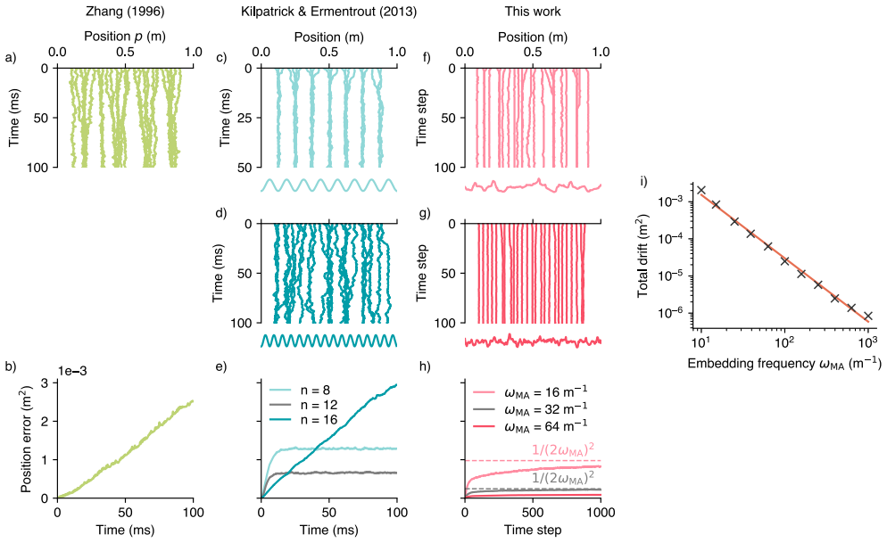
Simulate the network of the paper's experiments and sweep the embedding frequency $\omega_{\mathrm{MA}}$ while measuring the Hamming distance between adjacent discrete attractor states: the mechanism predicts this distance stays constant as the number of stable states grows, while a unimodal tiled attractor's distance shrinks, and a shrinking distance would mean diffusion returns. The second check is the drift exponent: if the RMS drift deviates from the reported $\omega_{\mathrm{MA}}^{-0.85}$ scaling and crosses into a random-walk regime at large $\omega_{\mathrm{MA}}$, the claim that resolution can be raised indefinitely without losing stability is falsified.
Extended reading notes
Core claim
The central claim is that the stability–resolution dilemma of continuous attractor networks disappears when the represented variable is encoded by multimodal periodic receptive fields of the form $x_i(p)=\mathbf{1}[\mathrm{mod}_L(\omega_i p+\theta_i)<1]$ — a sparse binary code in which each neuron is active at multiple locations spaced by its period, and blocks of neurons share a frequency with different phases, mirroring grid-cell modules. Under Hebbian covariance learning the random sampling noise of this embedding automatically roughens the energy landscape, with autocorrelation length $1/(2\omega_{\mathrm{MA}})$; the paper interprets this length as the effective spacing between discrete attractor states, so raising the mean-absolute embedding frequency $\omega_{\mathrm{MA}}$ adds resolvable stable states across the metre of track. Because each neuron now toggles twice per mode, the L1 path length of the code is $2N\,\omega_{\mathrm{MA}}/L$ rather than the at-most $2N$ of a bump code, so the added states sit at an unchanged Hamming distance in neural state space and diffusion is not reintroduced. The measured long-time RMS drift scales as $\omega_{\mathrm{MA}}^{-0.85}$, close to the ideal $\omega_{\mathrm{MA}}^{-1}$, and the same construction embeds planes, spheres, tori, and Möbius strips, with input-triggered integration along programmed vector fields and multiple maps stored in one network.
Load-bearing premise
The whole estimate of how finely the stable states are spaced rests on the assumption that the random error in the similarity between two position codes has the same statistics no matter how similar the two codes are; the paper calls this 'quite heavy-handed', it makes the predicted energy-fluctuation magnitude overshoot the simulations by about a factor of two, and if the error statistics actually depend strongly on state similarity, the predicted $1/(2\omega_{\mathrm{MA}})$ spacing — and with it the escape from the resolution–stability dilemma — collapses.
Editorial extensions
If this is right
- Raising the embedding frequency $\omega_{\mathrm{MA}}$ increases memory resolution without restoring diffusion, so stability and resolution stop being mutually exclusive; the paper demonstrates this against both the Zhang (1996) and Kilpatrick–Ermentrout (2013) baselines.
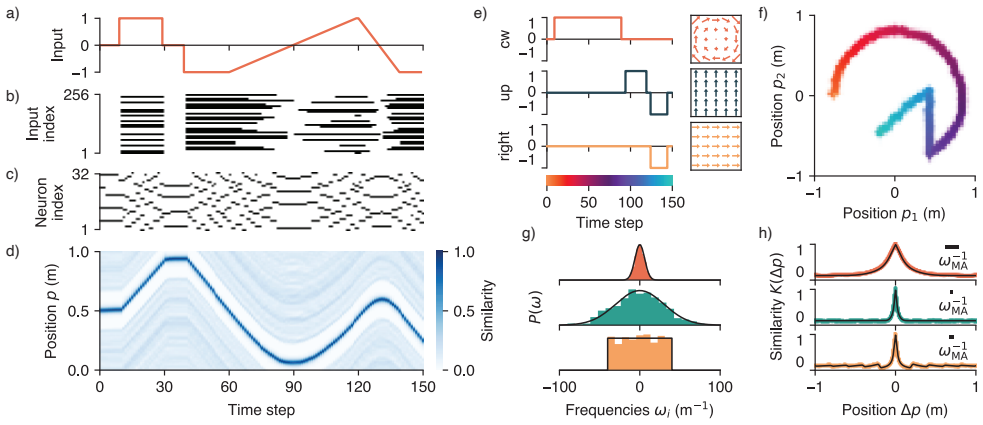
- The same Hebbian learning and block winner-take-all dynamics that store a line attractor store spheres, tori, and Möbius strips, and run input-triggered integration along freely programmed vector fields on those manifolds.
- Several environments can be stored in one network by superimposing separately generated weight matrices, with cross-talk between manifolds no worse than between distant points on a single manifold, and heteroassociative terms can switch between maps.
- Because the resolution ceiling is set by the code's path length, multimodal grid-cell-like codes support far finer working memories than unimodal place-cell-like codes at equal network size — the paper's answer to why entorhinal codes, not hippocampal place codes, should support continuous memory.
- The energy roughness that pins the states is not planted by hand: it arises automatically from finite-size sampling noise in the randomized embedding, with its length scale controlled by the frequency distribution $P(\omega)$.
Reading between the lines
- Reading the path-length argument as a design principle the paper leaves implicit: for any behavioural variable, the resolution a CAN can hold at fixed stability is set by how long a curve the code traces in neural state space, and codes with more modes per neuron extend that ceiling — a quantitative route to testing whether plane-wave codes suffer the intermediate trade-off the paper sketches but
- A testable dissociation for the entorhinal system: if the mechanism is right, grid modules with finer spacing should support sharper memory resolution while each stable state stays just as robust, so behavioural memory precision should track the finest available module rather than the population average.
- The graceful degradation under stochastically binarised weights seen in the manifold experiments suggests the scheme is a candidate for low-precision neuromorphic implementations of path integration, sidestepping the component-precision requirements usually blamed for CAN fragility.
- The reported factor-of-two gap between predicted and simulated energy covariance, with the length scale correct, points to a specific repair: weakening the independence assumption in the supplement by including the correlation between residual noise and kernel value should close most of the magnitude gap without moving the $1/(2\omega_{\mathrm{MA}})$ spacing.
Signed reviews
Editorial analysis
A structured set of objections, weighed in public.
Referee Report
Summary. The paper studies continuous attractor networks (CANs) that store a one-dimensional position variable and proposes replacing unimodal bump codes with sparse binary periodic ('grid-cell-like') embeddings x_i(p) = 1[mod_L(omega_i p + theta_i) < 1]. The central claim is that such multimodal codes increase the path length of the representation in neural state space, so that the number of discrete attractor states can grow with the mean embedding frequency omega_MA without reducing the neural-space distance between adjacent states; this is argued to escape the resolution-stability dilemma that limits unimodal CANs. The authors derive the expected similarity kernel, model residual inner-product errors as an Ornstein-Uhlenbeck process, and predict an energy-roughness autocorrelation length of 1/(2 omega_MA). Simulations show drift scaling approximately omega_MA^{-0.85} and stable memory at omega_MA up to 64, and the construction is extended to path integration, 2D plane attractors, curved manifolds, and multiple embedded manifolds.
Significance. If correct, the paper would provide a concrete mechanistic resolution of a long-standing dilemma in continuous attractor models, namely the trade-off between stability and resolution under noise and heterogeneity. The identification of representation path length as the controlling quantity is a useful conceptual contribution, and the explicit scaling predictions (e.g., the 1/(2 omega_MA) correlation length and the omega^{-0.85} drift) are falsifiable and largely confirmed by the accompanying simulations. The paper is also commendably explicit about the limitations of its analytic approximations, especially in Supplementary S3. The generalization to path integration and to manifolds of different topology extends the framework's potential impact beyond 1D memory. However, the central escape-from-diffusion claim is currently supported only over a finite frequency window and relies on an approximation whose quantitative accuracy is not fully established; the significance will hinge on whether the barrier-height scaling is addressed.
major comments (3)
- [Section II, 'Escaping the resolution-stability dilemma'; Fig. 1i; S3 Eq. (33)] The central claim that increasing omega_MA adds stable states without restoring diffusion is demonstrated only for omega_MA up to 64. The derived energy covariance in S3 Eq. (33), in the regime used here (N=4096, P omega_MA <= 64), has variance scaling as 1/omega_MA^2, so the energy-roughness amplitude scales as 1/omega_MA, and the typical energy barrier between adjacent minima spaced 1/(2 omega_MA) apart would be expected to shrink accordingly. The path-length argument fixes the Hamming distance between adjacent attractor states but does not establish that the barrier height remains above the effective noise temperature. Without an estimate of barrier height versus the noise floor, or diffusion measurements at substantially larger omega_MA (e.g., 128 and 256), the possibility remains that the resolution-stability dilemma is postponed rather than escaped. This is load-bearing for the paper's main claim and should be addressed directly.
- [Supplementary S3, 'Energy statistics'; Fig. S4] The theoretical derivation of the 1/(2 omega_MA) length scale rests on the explicitly acknowledged heavy-handed assumption that the residual inner-product error is described by the OU process (20) and is 'critically unaffected by the value of K.' This assumption is false for nearby states, where the error is exactly zero at Delta p = 0, and S4 shows that the predicted covariance magnitude is off by roughly a factor of two. The length-scale agreement in Fig. S4b is reassuring, but the covariance magnitude is exactly what would determine barrier heights. To make the central claim robust, the authors should either derive the energy statistics for the actual block-sparse process or provide a direct simulation-based check of the predicted barrier-height scaling, rather than relying on an approximation whose magnitude error is acknowledged.
- [Section IV, 'Comparison models'; Fig. 1a-e] The evidence that the new model escapes the dilemma is presented as a comparison with the Zhang (1996) and Kilpatrick-Ermentrout (2013) models under 'equal magnitudes of nonidealities.' The noise protocols are different (bit errors on the binary state versus clamped-current perturbations), and the statement that 1 ms of noise in the comparison models equals one time step in the new model is asserted rather than derived. If the effective perturbation strengths are not matched, the contrast in Fig. 1 could overstate the qualitative difference. Please quantify the equivalence (e.g., by measuring the free diffusion coefficient of each model with the roughness term removed) or soften the comparison.
minor comments (4)
- [Methods, Eq. (14) and S3 Eq. (33)] The main-text expression for the energy autocovariance, Eq. (14), and the supplementary expression, S3 Eq. (33), should be reconciled; the prefactors appear to differ by powers of L and P, and the definition of kappa_1 should be stated where Eq. (14) is introduced.
- [Section II, 'Escaping the resolution-stability dilemma'] The statement that the network can represent position to 'millimetre resolution' should be defined relative to the nominal state spacing 1/(2 omega_MA) and the observed RMS drift; with omega_MA = 64 over 1 m, the nominal spacing is about 7.8 mm, so 'millimetre' is not immediate from the stated parameters.
- [Supplementary S4, LCC binding relation] The LCC binding relation holds with probability 2/3 in the generic 'far' case; the paper should state how the 1/3 failure probability is handled in the 2D path-integration experiments (e.g., by the subsequent WTA cleanup), since this relation is used in the higher-dimensional constructions.
- [General] A data/code availability statement is missing; given the number of empirical claims, providing the simulation code would aid reproducibility.
Circularity Check
No significant circularity: the central scaling predictions are derived from the embedding/kernel statistics and verified in independent simulations.
full rationale
The paper's central claim—that increasing the mean-absolute embedding frequency ω_MA increases resolution without restoring diffusive instability—follows from two derived quantities: the energy autocorrelation length 1/(2ω_MA) (Supplementary S3, via the Ornstein-Uhlenbeck approximation of residual inner-product errors) and the growth of representation path length 2N·ω_MA/L (Section II). Both are consequences of the randomized periodic embedding (1) and its translation-invariant kernel (2)/(6), not fitted outputs or restatements of the desired conclusion. The measured RMS drift scaling ω_MA^{-0.85} is presented as an empirical result, and its deviation from the predicted ω_MA^{-1} is explicitly attributed to increased memory loading and interference; it is not used to fit the model. The 'quite heavy-handed' assumption in S3 that residual errors follow (20) regardless of the kernel value is a stated approximation, not a circular definition, and the paper itself reports that the energy-covariance magnitude is off by roughly a factor of two while the correlation length scale matches. Self-citations (Frady et al. 2022, 2023; Kymn et al. 2024b; Cotteret et al. 2024, 2025) support auxiliary machinery—VSA binding, LCC arithmetic, finite-state transitions—but the core line-attractor result and its 1D stability statistics are derived in this paper from the embedding model and verified with simulation. No target result is used as an input; no fitted parameter is renamed as a prediction; no load-bearing uniqueness claim is imported from the authors' prior work. The remaining question of whether stability persists at ω_MA values beyond those simulated is a regime-of-validity/robustness concern, not circularity.
Assumptions & free parameters
free parameters (6)
- Block size L =
8 (main text), 16 (Fig. S1)
- Mean-absolute embedding frequency ω_MA =
Varied, e.g., 16 and 64 m^-1 (Fig. 1)
- Surrogate steepness β =
5
- Integration speed constant c =
Not specified numerically
- Binarization steepness α =
5
- Bit error rate b =
10% per time step
assumptions (6)
- ad hoc to paper The residual inner-product error between two position states is modeled by the OU process (20) and is unaffected by the value of the kernel K.
- domain assumption Inner products between position states are well-approximated by their expected values in the auto-associative cleaning step.
- domain assumption The block-WTA operation can be implemented biologically by fast inhibition/divisive normalization.
- ad hoc to paper The LCC binding relation x(p)*_LCC x(q) ≈ x(p+q)*_LCC x(0) holds with probability 2/3 for far positions.
- ad hoc to paper Inverse energy weighting in Eq. (28) corrects higher-order curvature effects on state energies.
- standard math Noise effects on the attractor are reduced by a factor √N via attractor dynamics.
Cite this review
Pith. "Pith review of High-resolution spatial memory requires grid-cell-like neural codes." pith.science (2026). https://pith.science/paper/62Z7OMSU
@misc{pith2026250700598,
  author       = {Pith},
  title        = {Pith review of: High-resolution spatial memory requires grid-cell-like neural codes},
  year         = {2026},
  howpublished = {\url{https://pith.science/paper/62Z7OMSU}},
  note         = {Machine review of arXiv:2507.00598}
}
read the original abstract
Continuous attractor networks (CANs) are widely used to model how the brain temporarily retains continuous behavioural variables via persistent recurrent activity, such as an animal's position in an environment. However, this memory mechanism is very sensitive to even small imperfections, such as noise or heterogeneity, which are both common in biological systems. Previous work has shown that discretising the continuum into a finite set of discrete attractor states provides robustness to these imperfections, but necessarily reduces the resolution of the represented variable, creating a dilemma between stability and resolution. We show that this stability-resolution dilemma is most severe for CANs using unimodal bump-like codes, as in traditional models. To overcome this, we investigate sparse binary distributed codes based on random feature embeddings, in which neurons have spatially-periodic receptive fields. We demonstrate theoretically and with simulations that such grid-cell-like codes enable CANs to achieve both high stability and high resolution simultaneously. The model extends to embedding arbitrary nonlinear manifolds into a CAN, such as spheres or tori, and generalises linear path integration to integration along freely-programmable on-manifold vector fields. Together, this work provides a theory of how the brain could robustly represent continuous variables with high resolution and perform flexible computations over task-relevant manifolds.
Figures

Figures from the paper (1 more)

Reference graph
Works this paper leans on
-
[1]
a component for which xi(p) = 1 turns off, xi(p + δp) = 0
-
[2]
Z ∞ −∞ ¯K 2(p′)dp′ #2 = M 4 1 ω2 MA
a component for which xi(p) = 0 turns on, xi(p + δp) = 1. The change in overlap δXk is thus given by δXk = δX + k − δX − k δX + k ∼ B nk − Xk, ωk δp L − 1 δX − k ∼ B Xk, ωk δp 1 (13) where B(n, p) is the binomial distribution, and δX + k and δX − k are the number of neurons that switch on and off respectively. Ornstein-Uhlenbeck approximation In order to ...
work page 2010
-
[3]
Computing on functions using randomized vector representations (in brief)
These results are summarised by L N x(p) ∗LCC x(q) ∗−1 LCC x(0) · x(p + q) ≈ 1 if ωMAp ≈ 0 or ωMAq ≈ 0 1 2 else if ωMAp ≈ ±ωMAq 2 3 otherwise (45) and demonstrated in Fig. S5. An additional clean-up step with the help of an associative memory would then be needed, if one wanted to recover the summed hypervector x(p + q) exactly . Parameter Descrip...
-
[6]
For the case that p = −q, the equality to be satisfied is ⌊p′ + θ′⌋ + ⌊θ′ − p′⌋ = 0 (43) 9 4 2 0 2 4 Bound position p2 4 2 0 2 4 Comparison position p p1 = 1.7 a) b) 0.0 0.2 0.4 0.6 0.8 1.0 Similarity to comparison state 0.0 1.0 p1 = 1.7 0.0 1.0Similarity of correct state p1 = -1.2 4 2 0 2 4 Bound position p2 0.0 1.0 p1 = 3.4 1 MA Fig. S5: LCC binding wit...
-
[186]
Engineering recurrent neu- ral networks from task-relevant manifolds and dynam- ics
DOI: 10.1088/0954-898X/3/2/006. Plate, T. A. (1992). Holographic recurrent networks. In Advances in Neural Information Processing Systems (V ol. 5). Plate, T. A. (2003).Holographic Reduced Representation: Distributed Representation for Cognitive Structures . Pollock, E., & Jazayeri, M. (2020). “Engineering recurrent neu- ral networks from task-relevant ma...
arXiv 1992
-
[766]
Binding in hippocampal-entorhinal circuits enables compositionality in cognitive maps
DOI: 10.1038/s41583-022-00642-0. Kilpatrick, Z. P., & Ermentrout, B. (2013). “Wandering bumps in stochastic neural fields”. SIAM Journal on Applied Dynam- ical Systems, 12(1), 61–94. DOI: 10.1137/120877106. Kilpatrick, Z. P., Ermentrout, B., & Doiron, B. (2013). “Optimizing working memory with heterogeneity of recurrent cortical excitation”. The Journal o...
work page Pith review arXiv doi:10.48550/arxiv.2406.18808 2013
-
[1796]
Can we reconcile the declarative memory and spatial navigation views on hippocampal function?
DOI: 10.1152/jn.00005.2017. Eichenbaum, H., & Cohen, N. J. (2014). “Can we reconcile the declarative memory and spatial navigation views on hippocampal function?” Neuron, 83(4), 764–770. DOI: 10.1016/j.neuron.2014.07.032. Faisal, A. A., Selen, L. P. J., & Wolpert, D. M. (2008). “Noise in the nervous system”. Nature Reviews Neuroscience , 9(4), 292–303. DO...
Reviewed August 6, 2026 · model on record in the stance chip above.
Discussion (0). Continue with ORCID to comment.