REVIEW 3 major objections 4 minor 1 cited by
A theoretical prediction for the dipole in nearby distances using cosmography
T0 review · 3 major / 4 minor · reviewed 2026-08-06 · deepseek-v4-flash
Pith's one-line read The paper claims the dipole in luminosity distances of nearby sources can be predicted from gradients of the volume-smoothed expansion rate and matter density, with no background cosmology assumed, and shows the prediction matches fully…
desk verdict A useful, honestly-scoped validation of a smoothed cosmographic dipole prescription; the central averaging step is assumed and scale-tuned, so the 'prediction' label oversells it slightly. read the letter →
The pith
A machine-rendered reading of the paper's core claim, the machinery that carries it, and where it could break.
The reading
What carries the argument
The machinery is the generalized cosmographic expansion of the luminosity distance truncated at third order in redshift, combined with a smoothing step. The expansion's coefficients are generalized Hubble, deceleration, curvature, and jerk parameters defined along each line of sight; under quiet-universe assumptions these reduce, at the dipole level, to coefficients constructed from the spatial gradients of the volume-smoothed expansion rate $\langle\theta\rangle$ and density $\langle\rho\rangle$. Smoothing is performed with a Gaussian kernel whose width is matched to the redshift at which the dipole is evaluated, and the paper's test compares the resulting prediction with exact distances from geodesic ray tracing on the same constant-redshift spheres.
What would settle it
Run the same comparison in a simulation that resolves structure below the current fluid cutoff at roughly $8\,h^{-1}\mathrm{Mpc}$; if the predicted dipole from Eq. (8) does not track the ray-traced dipole to within ten percent at $z\lesssim0.02$, or if the residual does not shrink when the Gaussian width is varied across the tested $2\sigma$ to $4\sigma$ range, the smoothing-mapping assumption is falsified.
Extended reading notes
Core claim
The central claim is a calculational rule: the dipole of luminosity distance on constant-redshift spheres around a given comoving observer is, to third order in redshift, the direction-weighted sum of two gradient terms, $d_{L,\mathrm{dip}}(\mathbf{e},z) = e^\mu (d^{(2)}_{L,\mu} z^2 + d^{(3)}_{L,\mu} z^3)$, with $d^{(2)}_{L,\mu}$ proportional to $D_\mu\langle\theta\rangle/\langle\theta\rangle^3$ and $d^{(3)}_{L,\mu}$ receiving contributions from $D_\mu\langle\theta\rangle$ and $D_\mu\langle\rho\rangle$. These coefficients follow from the generalized cosmography of the luminosity distance in an arbitrary space-time, specialized to a pressureless dust congruence under the quiet-universe approximation. When tested in numerical relativity simulations with fully nonlinear ray tracing, the predicted dipole amplitude agrees with the ray-traced dipole to within about 10 percent for redshifts below 0.07 in a quasi-linear simulation and below 0.02 in a simulation with larger density contrasts; the predicted direction is typically aligned to better than 1 percent. This constitutes up to an order-of-magnitude improvement over the dipole extracted from the local, unsmoothed third-order cosmography.
Load-bearing premise
The load-bearing premise is that volume-smoothed averages of the expansion rate and density can be inserted into the nonlinear dipole coefficients and still predict the observed dipole, even though averaging and non-linear operations do not commute; the prediction also relies on the Gaussian smoothing scale being hand-matched to each redshift.
Editorial extensions
If this is right
- A measured low-redshift distance dipole can be interpreted as a signal of gradients in the large-scale expansion rate and density, without committing to a particular background cosmology.
- Because the third-order term is needed for the amplitude while the second-order term already gives the direction, fitting only the second-order dipole coefficient would yield a correct axis but an incorrect magnitude.
- On large smoothing scales the structure-induced dipole is suppressed and the ray-traced dipole becomes dominated by the observer's velocity relative to the average frame, so scale separates the two physical origins of the dipole.
- The framework is expected to extend to universe models containing a cosmological constant, since the derivation only requires the quiet-universe assumptions and the field equations, not the absence of dark energy.
- Applying this prediction to upcoming large low-redshift supernova samples would turn a nuisance anisotropy into a measurable cosmological signal.
Reading between the lines
- The optimal match between Gaussian smoothing scale and redshift is not fixed at 3 sigma, since the appendix shows the best match drifts to roughly 3.25-3.5 sigma at low redshift; a scale-dependent matching scheme is a natural extension that may push the 10 percent range farther.
- A more covariant volume average of the kind used in backreaction studies might repair the breakdown in the nonlinear simulation, because the paper attributes the failure to the naive averaged congruence not capturing kinematics on the averaging scale.
- The same averaging logic could be adapted to other dipolar observables, such as galaxy number counts or astrometric proper motions, where dipole excesses over the kinematic expectation have also been reported; the paper only hints at these directions.
- Combining the cosmographic gradient dipole with the kinematic boost dipole in one model could cover the intermediate redshifts $0.1\lesssim z\lesssim0.25$ where neither term alone fits, though the paper notes such a combination would require perturbation theory.
Editorial analysis
A structured set of objections, weighed in public.
Referee Report
Summary. This paper proposes a method to predict the dipolar anisotropy in the luminosity distance-redshift relation from smoothed cosmography. Using the third-order generalized cosmography of Heinesen, the authors write the dipole as Eq. (6) with coefficients constructed from gradients of the expansion rate and density. They replace the local fields θ and ρ by Gaussian-smoothed averages in Eq. (8), with the smoothing scale matched to the redshift of observation. The prediction is tested against fully relativistic ray-traced distances in two numerical-relativity simulations, one quasi-linear (L=2.56 h^-1 Gpc, N=256, λ_min=400 h^-1 Mpc) and one with more small-scale structure (L=3.072 h^-1 Gpc, λ_min=120 h^-1 Mpc). The authors report approximately 10% accuracy in dipole amplitude for z≲0.07 in the quasi-linear simulation and z≲0.02 in the more nonlinear simulation, with up to an order-of-magnitude improvement over unsmoothed local cosmography. They explicitly flag the assumed θ→⟨θ⟩ mapping as ambiguous and connect the smoothing question to the cosmological fitting problem.
Significance. The numerical comparison is a strength: the ray tracer solves the full geodesic and geodesic-deviation equations, the Richardson extrapolation in Appendix A indicates that numerical error is not the dominant source of mismatch for most observers, and the code is built on open-source components. If the averaging prescription can be justified or its error bounded, the method would provide a useful model-independent route to interpret low-redshift dipole measurements and connect them to expansion and density gradients. The paper is honest about the main caveat, that Eq. (8) assumes commutation of smoothing with nonlinear operations, but this caveat is exactly the load-bearing point. The current manuscript therefore establishes a promising phenomenological prescription rather than a fully derived theoretical prediction.
major comments (3)
- [§2.2, Eq. (8)] The central prediction is not derived: the replacement of θ and ρ by ⟨θ⟩ and ⟨ρ⟩ in the nonlinear ratios of Eq. (8) is stated as an assumption, and the text explicitly acknowledges that ⟨θ²⟩ is not equal to ⟨θ⟩². Because no controlled approximation quantifies the error introduced by this commutation, the agreement with the ray-traced dipole in Fig. 2 validates a chosen averaging prescription rather than a derived prediction. I request either a derivation or an estimate of the leading smoothing corrections, for example terms involving ⟨θ²⟩−⟨θ⟩², or an explicit reframing of Eq. (8) as a phenomenological ansatz whose accuracy is to be tested.
- [Appendix B; §3.4] The reported approximately 10% accuracy depends on a smoothing-to-redshift matching rule that is calibrated in the same analysis. Appendix B shows that the optimal matching lies between 3.25σ and 3.5σ at low redshift, and §5.1 states that the 3σ choice produces a slight negative bias. Since the same data are used to select the matching rule and to evaluate the prediction, the headline accuracy is partly post-hoc. Please present the dipole comparison for a fixed, prespecified matching rule across the full redshift range, and quantify how the accuracy changes over the 2.5σ to 4σ range shown in Fig. 10.
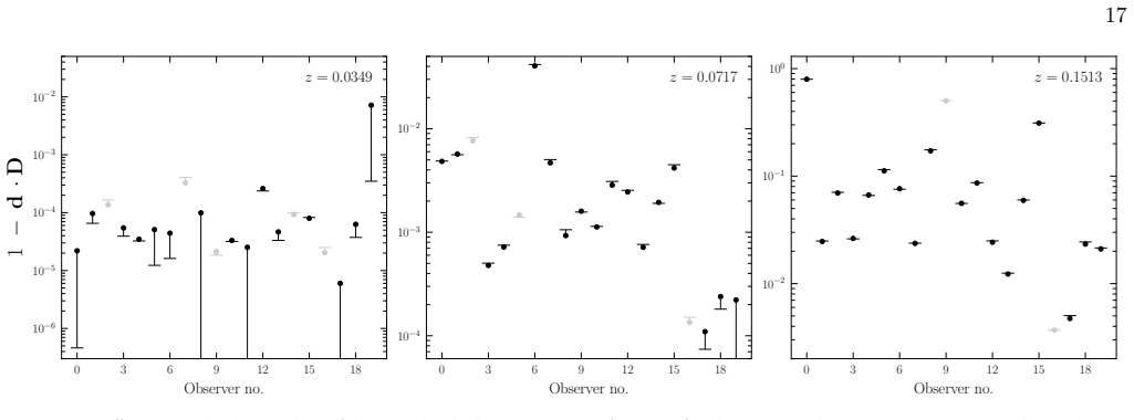
- [§5.3, Fig. 6] The validation is limited to quasi-linear universes: with the L=3.072 h^-1 Gpc simulation, which has typical density contrast around 0.05, the prediction reaches 10% accuracy only for z≲0.02, and the direction is matched to 1% only at even lower redshifts. The paper acknowledges this limitation and relates it to the fitting problem, but the abstract's claim of an order-of-magnitude improvement is based on the smoother simulation. I recommend making this quasi-linear scope explicit in the abstract and conclusions, and stating clearly that no claim is made for the deeply nonlinear regime.
minor comments (4)
- [Fig. 1 caption] The caption gives the simulation size as L=2.56 h^-1 Mpc; from Section 3.3 this should be h^-1 Gpc.
- [Fig. 5 caption] Typo: 'comsography' should be 'cosmography'.
- [Footnote 9, §4.1] The ray-tracing part of mescaline is not yet public; please include a code and data availability statement with a timeline or repository to support reproducibility.
- [§3.3] The choice h=0.45, rather than the Planck value used for the power spectrum, is unusual; a sentence explaining that this is a simulation scale choice and does not affect the model-independent prediction would help.
Circularity Check
The smoothed-cosmography dipole prediction is partially calibrated: the 3-sigma smoothing-scale-to-redshift mapping is chosen in Appendix B by comparison with the ray-traced dipole, so the reported ~10% agreement is in-sample for that parameter.
-
fitted input called prediction
[Section 3.4 (Eq. 12-13) and Appendix B]
"We smooth these quantities using a Gaussian kernel with a 3–σ width that coincides with the redshift of interest (in Appendix B we show that this is the optimal choice for matching smoothing scale with redshift). ... In the main text, we have chosen to match the 3–σ width of the Gaussian kernel to an approximate redshift by comparing the predicted dipole to the ray-traced dipole."
The smoothing scale is the method's free parameter, and Appendix B fixes it by comparing the predicted dipole to the ray-traced dipole, which is the same benchmark used to claim ~10% agreement. The reported accuracy is therefore not an out-of-sample test of a parameter-free prediction: the 3-sigma matching is calibrated to minimize the discrepancy on the target data. The dipole amplitude itself is still computed from smoothed theta and rho gradients, so this is a partial, not a complete, reduction of the prediction to its inputs.
full rationale
The core dipole formula (8) is constructed from smoothed expansion-rate and density gradients, and the ray-traced luminosity distances provide an external, independent benchmark; the dipole amplitude is not fitted to that benchmark. The main circular element is the choice of the Gaussian smoothing scale: Appendix B explicitly selects the 3-sigma scale-to-redshift mapping by comparing prediction with the ray-traced dipole, so the headline 'within ~10%' accuracy is partially in-sample. The paper also relies on the authors' earlier derivation of the dipole coefficients (7) and on an explicitly assumed, acknowledged-ambiguous replacement of local fields by smoothed averages, since the text notes that <theta^2> is not equal to <theta>^2; these are correctness and provenance concerns rather than circular reductions, because the earlier derivation is not fitted to the present target and the averaging assumption is stated openly. Considering the external validation and the fact that the dipole signal itself is not fitted, the circularity is mild.
Assumptions & free parameters
free parameters (3)
- Smoothing-to-redshift matching width (n-sigma of Gaussian) =
3 sigma (chosen as optimal over 2 sigma to 4 sigma)
- Gaussian kernel FWHM in grid cells =
4, 8, 12, 16 dx for the L=2.56 h^-1 Gpc run; 10 grid cells minimum for the L=3.072 h^-1 Gpc run
- Initial power spectrum cutoff lambda_min =
400 h^-1 Mpc for the smooth run, 120 h^-1 Mpc for the more nonlinear run
assumptions (5)
- domain assumption Einstein's general relativity holds, with dust matter described by T_mu nu = rho u_mu u_nu at leading order.
- domain assumption Quiet universe approximation: pressureless dust, vorticity-free, small shear and electric Weyl compared to expansion, while gradients of shear and electric Weyl can be comparable to gradients of expansion and density.
- ad hoc to paper The mapping theta to <theta> and rho to <rho> is valid at lowest order for predicting observables.
- domain assumption Gaussian smoothing on a spatially flat slice is a valid proxy for the average congruence.
- domain assumption The EdS distance-redshift relation with H0=<theta>/3 translates a smoothing scale to a redshift.
Cite this review
Pith. "Pith review of A theoretical prediction for the dipole in nearby distances using cosmography." pith.science (2026). https://pith.science/paper/XQNGOEER
@misc{pith2026250701095,
  author       = {Pith},
  title        = {Pith review of: A theoretical prediction for the dipole in nearby distances using cosmography},
  year         = {2026},
  howpublished = {\url{https://pith.science/paper/XQNGOEER}},
  note         = {Machine review of arXiv:2507.01095}
}
abstract
Cosmography is a widely applied method to infer kinematics of the Universe at small cosmological scales while remaining agnostic about the theory of gravity at play. Usually cosmologists invoke the Friedmann-Lemaitre-Robertson-Walker (FLRW) metric in cosmographic analyses, however generalised approaches allow for analyses outside of any assumed geometrical model. These methods have great promise to be able to model-independently map the cosmic neighborhood where the Universe has not yet converged to isotropy. In this regime, anisotropies can bias parameter inferences if they are not accounted for, and thus must be included for precision cosmology analyses, even when the principle aim is to infer the background cosmology. In this paper, we develop a method to predict the dipole in luminosity distances that arises due to nearby inhomogeneities. This is the leading-order correction to the standard isotropic distance-redshift law. Within a very broad class of general-relativistic universe models, we provide an interpretation of the dipole in terms of the gradients in expansion rate and density which is free from any underlying background cosmology. We use numerical relativity simulations, with improved initial data methods, alongside fully relativistic ray tracing to test the power of our prediction. We find our prediction accurately captures the dipole signature in our simulations to within ~10% for redshifts $z\lesssim 0.07$ in reasonably smooth simulations. In the presence of more non-linear density fields, we find this reduces to $z\lesssim 0.02$. This represents up to an order of magnitude improvement with respect to what is achieved by naive, local cosmography-based predictions. Our paper thus addresses important issues regarding convergence properties of anisotropic cosmographic series expansions that would otherwise limit their applicability to very narrow redshift ranges.
Figures


Figures from the paper (8 more)




Forward citations
Cited by 1 Pith paper
-
Cosmography for a General Spacetime Centred at Arbitrary Redshift
A general-relativistic cosmographic expansion centered at arbitrary redshift is derived and tested on void and overdensity LTB models, showing that its coefficients lose strict local meaning near density gradients.
Reference graph
Works this paper leans on
-
[1]
Abdalla E et al. 2022JHEAp34, 49–211. Abghari A, Bunn E F, Hergt L T, Li B, Scott D, Sullivan R M and Wei D 2024J. Cosmology Astropart. Phys.2024(11),
work page 2024
-
[13]
Maartens R, Santiago J, Clarkson C, Kalbouneh B and Marinoni C 2024J. Cosmology Astropart. Phys.2024(9),
work page 2024
-
[25]
Dhawan S, Borderies A, Macpherson H J and Heinesen A 2023 Mon. Not. Roy. Astron. Soc.519(4), 4841–4855. Dunsby P K S, Bassett B A C C and Ellis G F R 1997Classical and Quantum Gravity14(5), 1215–1222. Ehlers J 1993General Relativity and Gravitation 25(12), 1225–1266. Ellis G F R 2009General Relativity and Gravitation 41(3), 581–660. Ellis G F R and Baldwi...
work page Pith review arXiv 2023
-
[34]
Bonvin C, Durrer R and Kunz M 2006Phys. Rev. Lett. 96, 191302. Brown D, Diener P, Sarbach O, Schnetter E and Tiglio M 2009 Phys. Rev. D79(4), 044023. Bruni M, Matarrese S and Pantano O 1995ApJ445,
work page 2009
-
[43]
Löffler F, Faber J, Bentivegna E, Bode T, Diener P, Haas R, Hinder I, Mundim B C, Ott C D, Schnetter E, Allen G, Campanelli M and Laguna P 2012Classical and Quantum Gravity29(11), 115001. LSST Science Collaboration, Abell P A, Allison J, Anderson S F, Andrew J R, Angel J R P, Armus L, Arnett D, Asztalos S J, Axelrod T S, Bailey S et al. 2009arXiv e-prints...
-
[53]
Anchordoqui L A, Di Valentino E, Pan S and Yang W 2021 JHEAp32, 28–64
Aluri P k, Cea P, Chingangbam P, Chu M C, Clowes R G, Hutsemékers D, Kochappan J P, Lopez A M, Liu L, Martens N C M, Martins C J A P, Migkas K, Ó Colgáin E, Pranav P, Shamir L, Singal A K, Sheikh-Jabbari M M, Wagner J, Wang S J, Wiltshire D L, Yeung S, Yin L and Zhao W 2023Classical and Quantum Gravity40(9), 094001. Anchordoqui L A, Di Valentino E, Pan S ...
work page 2021
-
[56]
Cattoen C and Visser M 2007Class. Quant. Grav.24, 5985–5998. Clarkson C, Ellis G F R, Faltenbacher A, Maartens R, Umeh O and Uzan J P 2012Mon. Not. Roy. Astron. Soc. 426, 1121–1136. Clarkson C, Ellis G, Larena J and Umeh O 2011Reports on Progress in Physics74(11), 112901. Clarkson C and Maartens R 2010Classical and Quantum Gravity 27(12), 124008. Clarkson...
-
[67]
Adamek J, Clarkson C, Durrer R, Heinesen A, Kunz M and Macpherson H J 2024Open J
Adamek J, Barrera-Hinojosa C, Bruni M, Li B, Macpherson H J and Mertens J B 2020Classical and Quantum Gravity 37(15), 154001. Adamek J, Clarkson C, Durrer R, Heinesen A, Kunz M and Macpherson H J 2024Open J. Astrophys.7, 001c.118782. Adamek J, Daverio D, Durrer R and Kunz M 2016J. Cosmology Astropart. Phys.2016(7),
work page 2016
Show all 16 references
-
[68]
Sanghai V A A and Clifton T 2015Phys. Rev. D91, 103532. [Erratum: Phys.Rev.D 93, 089903 (2016)]. Sarma M, Marinoni C, Kalbouneh B, Clarkson C and Maartens R
2016
-
[69]
arXiv:2510.02510
Kalbouneh B, Marinoni C, Maartens R, Bel J, Santiago J, Clarkson C, Sarma M and Virey J 2025 p. arXiv:2510.02510. Kalbouneh B, Santiago J, Marinoni C, Maartens R, Clarkson C and Sarma M 2025JCAP02,
2025
-
[70]
MacCallum M A H and Ellis G F R 1970Comm. Math. Phys. 19, 31–64. Macpherson H J 2023J. Cosmology Astropart. Phys. 2023(3),
2023
-
[76]
Koksbang S M 2025Phys. Rev. D111(12), 123516. Kristian J and Sachs R K 1966Astrophys. J.143, 379–399. Lesgourgues J 2011arXiv e-printsp. arXiv:1104.2932. Lewis A and Bridle S 2002Phys. Rev. D66(10), 103511. Lobo F S N, Mimoso J P and Visser M 2020JCAP04,
-
[111]
Macpherson H J and Heinesen A 2021Phys. Rev. D104, 023525. [Erratum: Phys.Rev.D 104, 109901 (2021)]. Macpherson H J, Lasky P D and Price D J 2017Phys. Rev. D 95(6), 064028. Macpherson H J, Lasky P D and Price D J 2018Astrophys. J. 865(1), L4. Macpherson H J, Price D J and Lask...
2021
-
[112]
2020A&A641, A6
Planck Collaboration, Aghanim N, Akrami Y, Ashdown M, Aumont J, Baccigalupi C, Ballardini M, Banday A J, Barreiro R B, Bartolo N, Basak S et al. 2020A&A641, A6. Planck Collaboration, Aghanim N, Armitage-Caplan C, Arnaud M, Ashdown M, Atrio-Barandela F, Aumont J, Baccigalupi C,...
2019
-
[279]
The influence of structure formation on the evolution of the universe
Umeh O 2013 "The influence of structure formation on the evolution of the universe." PhD thesis University of Cape Town, Faculty of Science, Department of Mathematics and Applied Mathematics. 21 van Elst H 1996 Extensions and applications of 1+3 decomposition methods in genera...
2013
-
[2025]
Rept.984, 1–55
Schöneberg N, Franco Abellán G, Pérez Sánchez A, Witte S J, Poulin V and Lesgourgues J 2022Phys. Rept.984, 1–55. Secrest N J, von Hausegger S, Rameez M, Mohayaee R and Sarkar S 2022ApJ937(2), L31. Secrest N J, von Hausegger S, Rameez M, Mohayaee R, Sarkar S and Colin J 2021ApJ...
2023
Reviewed August 6, 2026 · model on record in the stance chip above.
Discussion (0). Continue with ORCID to comment.