REVIEW 3 major objections 4 minor 91 references
Tensor network methods for the Gross-Pitaevskii equation on fine grids
T0 review · 3 major / 4 minor · reviewed 2026-08-06 · deepseek-v4-flash
Pith's one-line read Tensor networks make Gross-Pitaevskii simulations possible on grids direct solvers cannot reach.
desk verdict Useful first demonstration of MPS-GPE with QFT-MPO and honest benchmarks, but the headline log-scaling claim ignores the phase MPOs and is likely unestablished in the fine-grid regime the paper motivates. read the letter →
The pith
A machine-rendered reading of the paper's core claim, the machinery that carries it, and where it could break.
The reading
What carries the argument
The central object is the QFT-MPO: a matrix product operator representation of the quantum Fourier transform built from a tensor network of single-qubit Hadamard gates and controlled rotations. A matrix product state is a chain of tensors connected by bonds; the bond dimension $\chi$ controls how much correlation can be represented, so truncating singular values gives physically motivated data compression. The QFT-MPO carries the argument because kinetic-energy steps become diagonal multiplications in momentum space, and because its bond dimension saturates at a small constant (around 10 in 1D and for the sequential ordering in 2D) even when the grid is exponentially refined. Its application costs $O(N\chi^2)$ per Fourier transform, and the nonlinear term $|\Psi|^2$ dominates the per-step cost at $O(N\chi^4)$, giving the overall $O(\chi^4 \log M)$ scaling.
What would settle it
Run the QFT-MPO split-step method on forced quantum turbulence on $128^3$ and $256^3$ grids and record the maximum bond dimension needed for a fixed truncation error; the central claim is falsified if $\chi$ must double when the linear grid size doubles, since the cost then scales no better than a direct solver.
Extended reading notes
Core claim
The authors establish that a matrix product state can encode solutions of the Gross-Pitaevskii equation with enough compression to make very fine grids practical, provided the state has restricted correlations. The central technical discovery is that the quantum Fourier transform can be implemented as a matrix product operator with bond dimension that does not grow with grid size: omitting the final bit-reversal step leaves an operator with exponentially decaying singular values, so the whole spectral split-step method can be run as MPS contractions. They verify this against analytic soliton solutions and against direct spectral simulations for vortex shedding, and they show that the maximum bond dimension stays in the tens during vortex formation, while the storage cost at a fixed bond dimension scales linearly in the MPS length, i.e. logarithmically in grid count. The same Fourier-based construction handles the nonlocal dipolar interaction as a convolution, with the interaction kernel's bond dimension growing only logarithmically with the MPS length. The paper concludes that for problems whose dynamics produce modest bond dimension, fine-grid cold-atom simulations, including 3D cases beyond $128^3$, become feasible.
Load-bearing premise
The whole speedup rests on the assumption that the condensate wavefunction can be represented by a matrix product state of small bond dimension; if correlations grow steeply with system size or time, the $O(\chi^4 \log M)$ advantage over direct simulation disappears.
Editorial extensions
If this is right
- At a fixed bond dimension, computer time grows only linearly with the length of the matrix product state, so doubling the linear grid resolution adds a small constant cost instead of an eightfold cost in 3D.
- The compression ratio, measured as MPS parameters over direct-simulation parameters, improves exponentially as grids get finer; a 3D $128^3$ simulation with $\chi=64$ stores only about 4% of the direct-simulation data.
- Split-step evolution with the QFT-MPO outperforms finite-difference RK4 in the tests, and fourth-order Trotter splitting allows larger time steps at similar or better accuracy.
- Dipolar interactions, evaluated as a Fourier convolution, keep their representation cost logarithmic in grid count, so short-range dipole physics is accessible on finer grids.
- The results provide a route to quantum-turbulence simulations with far better spatial resolution than direct numerical simulation, assuming the state's bond dimension stays bounded.
Reading between the lines
- Editorial inference: the QFT-MPO construction transfers to any nonlinear Schr\"odinger-type equation solved spectrally, so nonlinear optics and plasma models with similar structure could inherit the same logarithmic scaling.
- Editorial inference: the method turns the bond dimension itself into a diagnostic of correlation structure; watching $\chi(t)$ across vortex-shedding and turbulence transitions could reveal when the compressible, low-entanglement description breaks down.
- Editorial inference: a concrete stress test would be forced quantum turbulence with energy injected at large scales: the central claim survives only if the required $\chi$ grows more slowly than the grid count, so measuring $\chi$ at $256^3$ versus $128^3$ would settle the practical range.
Editorial analysis
A structured set of objections, weighed in public.
Referee Report
Summary. The paper develops matrix-product-state (MPS) based solvers for the Gross-Pitaevskii equation and its dissipative and dipolar generalizations. The central technical ingredient is a matrix-product-operator representation of the quantum Fourier transform, which allows a spectral (split-step) treatment of the kinetic term with an operator bond dimension that saturates as the grid is refined. The authors benchmark the method against an analytic bright-soliton solution and against XMDS2 direct numerical simulations for vortex shedding in two dimensions, and also present three-dimensional vortex-shedding simulations and a dipolar-gas rotation example. The central claim is that, for states with sufficiently small bond dimension, the computational cost scales as O(χ^4 log M) in the number of grid points M, enabling fine-grid simulations that would be impractical with direct numerical simulation.
Significance. If the central scaling claim holds, the paper would provide a useful new tool for cold-atom simulations where a wide range of length scales must be resolved, such as quantum turbulence and short-range dipolar interactions. The manuscript is noticeably stronger than a pure proposal: it includes quantitative error benchmarks against an analytic solution and against an independent direct solver, convergence checks over truncation cutoff and grid size, and explicit CPU-time versus grid-size measurements. The paper also honestly acknowledges, in the conclusion, that the achievable compression is physics-dependent and must be tested for each problem instance. The main reservation is that the central asymptotic cost claim is not yet supported by an analysis of all operators entering the split-step scheme, and the extrapolation to the very large grids invoked in the motivation goes beyond the sizes for which accuracy is demonstrated.
major comments (3)
- [Section II.B and Eq. (13)] This is the load-bearing point for the central logarithmic-scaling claim, and the omission needs to be addressed before the claim can be accepted as stated.
- [Section III.C] This comment is proportionate because the abstract and introduction emphasize turbulent dynamics, where the 3D demonstration is the most relevant evidence.
- [Section III.B.1, Fig. 14] This is not a request for a new research program; it is a request for consistency between the data actually shown and the strength of the claims made from it.
minor comments (4)
- [Section IV.A and Conclusion] The text in Section IV.A says the dipolar-interaction MPO bond dimension 'appears to scale logarithmically with MPS length,' while the Conclusion says it 'scales linearly in MPS length.' These statements are inconsistent as written; since M grows as 2^N, one of them is presumably intended to refer to log M, and the wording should be corrected.
- [General] The manuscript does not include a data-availability or code-availability statement. Releasing the MPS simulation code would substantially strengthen reproducibility, given the algorithmic detail that is necessarily compressed into the text.
- [Section II.B, Eq. (17)] The notation in Eq. (17) defines a, b_n, and c_n, but the three tensors are not clearly labeled in Fig. 2, and the contraction order is described only verbally. A short explicit formula for the full QFT-MPO tensor network would help readers implement or verify the construction.
- [Abstract and Introduction] The phrase 'an indispensable tool' in the first sentence of the Introduction contains a typo ('an' should be 'a'). Minor typographical errors of this kind appear in several places, including 'representat' in Section I.B and 'propigation' in the caption of Fig. 8.
Circularity Check
No significant circularity: the method is benchmarked against external analytic and direct numerical references, and the central scaling claims are not fitted to the target results.
full rationale
The paper's central claim is that tensor network simulations of the Gross-Pitaevskii equation can achieve O(χ^4 log M) scaling and exponential data compression when the solution is well represented by a low-bond-dimension MPS. This claim is not derived from a self-referential loop. The accuracy of the method is checked against two independent external benchmarks: the analytic bright-soliton solution, via the error defined in Eq. (21), and direct numerical simulation using the XMDS2 package, via the error defined in Eq. (22). These comparisons are genuine external validations because no free parameters are fitted to the target simulation results; the only adjustable parameters are the truncation cutoff and bond dimension, which are convergence parameters, not fitted outputs. The QFT-MPO construction is imported from Ref. [42], which is an external prior result and is used as a tool; the paper's own contribution is the application to the GPE, and the efficiency of the QFT-MPO is separately measured in Figs. 3 and 5 rather than assumed from the target dynamics. The dipolar interaction kernels are taken from published formulas, and their MPS bond dimensions are measured directly by SVD truncation. The paper also explicitly acknowledges the limitation that the achievable compression depends on the physics of each instance, stating in the conclusion that 'the data compression one can achieve with tensor networks for a given problem will depend upon the physics of that instance.' This is an honest scope condition rather than a circular justification. The concern that the bond dimension of the phase operators in the split-step scheme is not analyzed is a correctness or completeness risk, not a circularity: it challenges an assumption about compressibility, but the paper does not define the claimed scaling in terms of the data it predicts. No self-citation is load-bearing, no fitted parameter is renamed as a prediction, and no known result is merely renamed. Therefore the derivation chain is self-contained against external benchmarks, and the appropriate circularity score is 0.
Assumptions & free parameters
assumptions (4)
- domain assumption The GPE with phenomenological damping models BEC dynamics.
- domain assumption The core QFT without final qubit reversal can serve as the Fourier transform in split-step methods.
- standard math Trotter-Suzuki decomposition error bounds apply to the non-unitary modified GPE evolution operator.
- domain assumption Singular value truncation of MPS preserves accuracy within cutoff for studied dynamics.
Cite this review
Pith. "Pith review of Tensor network methods for the Gross-Pitaevskii equation on fine grids." pith.science (2026). https://pith.science/paper/XBJOSDOY
@misc{pith2026250701149,
  author       = {Pith},
  title        = {Pith review of: Tensor network methods for the Gross-Pitaevskii equation on fine grids},
  year         = {2026},
  howpublished = {\url{https://pith.science/paper/XBJOSDOY}},
  note         = {Machine review of arXiv:2507.01149}
}
read the original abstract
The Gross-Pitaevskii equation and its generalisations to dissipative and dipolar gases have been very useful in describing dynamics of cold atomic gases, as well as polaritons and other nonlinear systems. For some of these applications the numerically accessible grid spacing can become a limiting factor, especially in describing turbulent dynamics and short-range effects of dipole-dipole interactions. We explore the application of tensor networks to these systems, where (in analogy to related work in fluid and plasma dynamics), they allow for physically motivated data compression that makes simulations possible on large spatial grids which would be unfeasible with direct numerical simulations. Analysing different non-equilibrium cases involving vortex formation, we find that these methods are particularly efficient, especially in combination with a matrix product operator representation of the quantum Fourier transform, which enables a spectral approach to calculation of both equilibrium states and time-dependent dynamics. The efficiency of these methods has interesting physical implications for the structure in the states that are generated by these dynamics, and provides a path to describe cold gas experiments that are challenging for existing methods.
Figures


Figures from the paper (22 more)




Reference graph
Works this paper leans on
-
[1]
This external potential, Vpad(x, t), which we call a ‘paddle’, has a fixed, rectan- gular shape, and is moved across the BEC with a sweep velocity v (see Fig
Single Paddle We use our MPS based methods to now study the dynamics of a BEC when a strong external potential is swept through the system. This external potential, Vpad(x, t), which we call a ‘paddle’, has a fixed, rectan- gular shape, and is moved across the BEC with a sweep velocity v (see Fig. 10). To have a resemblance closer to that which occurs exp...
-
[2]
We consider an alter- native stirring mechanism, replacing the one large paddle with four smaller paddles, all aligned along the y direc- tion
Multiple paddles Having demonstrated and bench-marked the ability of one to use tensor networks to perform simulations of the GPE in the previous sections, we now use our tensor network approach to further probe vortex dynamics and interactions in the modified GPE. We consider an alter- native stirring mechanism, replacing the one large paddle with four s...
2024
-
[3]
J. D. Biamonte and V. Bergholm, arXiv: Quantum Physics (2017)
2017
-
[4]
Or´ us, Nat Rev Phys1, 538–550 (2019)
R. Or´ us, Nat Rev Phys1, 538–550 (2019)
2019
-
[5]
Or´ us, Annals of Physics349, 117–158 (2014)
R. Or´ us, Annals of Physics349, 117–158 (2014)
2014
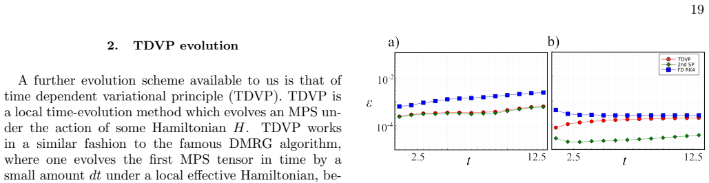
-
[6]
Schollw¨ ock, Annals of Physics326, 96–192 (2011)
U. Schollw¨ ock, Annals of Physics326, 96–192 (2011)
2011
-
[7]
G. K.-L. Chan, A. Keselman, N. Nakatani, Z. Li, and S. R. White, Matrix product operators, matrix product states, and ab initio density matrix renor- malization group algorithms (2016), arXiv:1605.02611 [physics.chem-ph]. 17
work page Pith review arXiv 2016
-
[8]
Paeckel, T
S. Paeckel, T. K¨ ohler, A. Swoboda, S. R. Manmana, U. Schollw¨ ock, and C. Hubig, Annals of Physics 411, 167998 (2019)
2019
Show all 91 references
-
[9]
Vanderstraeten, J
L. Vanderstraeten, J. Haegeman, and F. Verstraete, Sci- Post Physics Lecture Notes 10.21468/scipostphyslect- notes.7 (2019)
2019 doi
-
[10]
Haegeman, C
J. Haegeman, C. Lubich, I. Oseledets, B. Vandereycken, and F. Verstraete, Physical Review B 94, 10.1103/phys- revb.94.165116 (2016)
2016 doi
-
[11]
Evenbly and G
G. Evenbly and G. Vidal, Journal of Statistical Physics 145, 891–918 (2011)
2011
-
[12]
Cichocki, Tensor networks for big data ana- lytics and large-scale optimization problems (2014), arXiv:1407.3124 [cs.NA]
A. Cichocki, Tensor networks for big data ana- lytics and large-scale optimization problems (2014), arXiv:1407.3124 [cs.NA]
2014 arXiv
-
[13]
Schuch, M
N. Schuch, M. M. Wolf, F. Verstraete, and J. I. Cirac, Phys. Rev. Lett. 100, 030504 (2008)
2008
-
[14]
Iblisdir, R
S. Iblisdir, R. Or´ us, and J. I. Latorre, Phys. Rev. B 75, 104305 (2007)
2007
-
[15]
Hong, Y.-X
R. Hong, Y.-X. Xiao, J. Hu, A.-C. Ji, and S.-J. Ran, Phys. Rev. B 105, 165116 (2022)
2022
-
[16]
et.al, Nat Comput Sci 2, 30–37(2022)
N. et.al, Nat Comput Sci 2, 30–37(2022)
2022
- [17]
-
[18]
Ye and N
E. Ye and N. F. G. Loureiro, Physical Review E 106, 10.1103/physreve.106.035208 (2022)
2022 doi
-
[19]
Lubasch, P
M. Lubasch, P. Moinier, and D. Jaksch, Journal of Com- putational Physics 372, 587–602 (2018)
2018
-
[20]
Ye and N
E. Ye and N. Loureiro, Quantized tensor net- works for solving the vlasov-maxwell equations (2024), arXiv:2311.07756 [physics.comp-ph]
2024 arXiv
-
[21]
Gourianov, P
N. Gourianov, P. Givi, D. Jaksch, and S. B. Pope, Tensor networks enable the calculation of turbulence probability distributions (2024), arXiv:2407.09169 [physics.flu-dyn]
2024 arXiv
-
[22]
H¨ olscher, P
L. H¨ olscher, P. Rao, L. M¨ uller, J. Klepsch, A. Luckow, T. Stollenwerk, and F. K. Wilhelm, Quantum-inspired fluid simulation of 2d turbulence with gpu acceleration (2024), arXiv:2406.17823 [physics.flu-dyn]
2024
-
[23]
Pethick, Bose-Einstein condensation in dilute gases , second edition
C. Pethick, Bose-Einstein condensation in dilute gases , second edition.. ed. (Cambridge University Press, Cam- bridge, 2008)
2008
-
[24]
Pitaevskii and S
L. Pitaevskii and S. Stringari, Bose-Einstein condensa- tion and superfluidity (Oxford University Press, 2016) pp. 42–65
2016
-
[25]
Proukakis, S
N. Proukakis, S. Gardiner, M. Davis, and M. Szyma´ nska, Quantum Gases (IMPERIAL COLLEGE PRESS, 2013) https://www.worldscientific.com/doi/pdf/10.1142/p817
2013 doi
-
[26]
Blakie, A
P. Blakie, A. Bradley, M. Davis, R. Ballagh, and C. Gardiner, Advances in Physics 57, 363 (2008), https://doi.org/10.1080/00018730802564254
2008 doi
-
[27]
T. Z. Fischer and A. S. Bradley, Regimes of steady-state turbulence in a quantum fluid (2024), arXiv:2409.03184 [cond-mat.quant-gas]
2024 arXiv
-
[28]
Kobayashi, P
M. Kobayashi, P. Parnaudeau, F. Luddens, C. Lothod´ e, L. Danaila, M. Brachet, and I. Danaila, Computer Physics Communications 258, 107579 (2021)
2021
-
[30]
A. W. Baggaley and N. G. Parker, Physical Review A 97, 10.1103/physreva.97.053608 (2018)
2018 doi
-
[31]
Hern´ andez-Rajkov, N
D. Hern´ andez-Rajkov, N. Grani, F. Scazza, G. Del Pace, W. J. Kwon, M. Inguscio, K. Xhani, C. Fort, M. Mod- ugno, F. Marino, and G. Roati, Nature Physics 20, 939–944 (2024)
2024
-
[32]
E. Poli, D. Baillie, F. Ferlaino, and P. B. Blakie, Excitations of a two-dimensional supersolid (2024), arXiv:2407.01072 [cond-mat.quant-gas]
2024 arXiv
-
[33]
B. T. E. Ripley, D. Baillie, and P. B. Blakie, Phys. Rev. A 108, 053321 (2023)
2023
-
[34]
Bland, G
T. Bland, G. Lamporesi, M. J. Mark, and F. Ferlaino, Comptes Rendus. Physique 24, 133–152 (2024)
2024
-
[35]
Sabari, R
S. Sabari, R. Kishor Kumar, and L. Tomio, Phys. Rev. A 109, 023313 (2024)
2024
-
[36]
Gauthier, M
G. Gauthier, M. T. Reeves, X. Yu, A. S. Bradley, M. A. Baker, T. A. Bell, H. Rubinsztein-Dunlop, M. J. Davis, and T. W. Neely, Science 364, 1264–1267 (2019)
2019
-
[37]
Y. P. Sachkou, C. G. Baker, G. I. Harris, O. R. Stockdale, S. Forstner, M. T. Reeves, X. He, D. L. McAuslan, A. S. Bradley, M. J. Davis, and W. P. Bowen, Science 366, 1480–1485 (2019)
2019
-
[38]
Y. L. et al, New Journal of Physics 24, 10.1088/1367- 2630/ac8656 (2022)
2022 doi
-
[39]
Navon, C
N. Navon, C. Eigen, J. Zhang, R. Lopes, A. L. Gaunt, K. Fujimoto, M. Tsubota, R. P. Smith, and Z. Hadz- ibabic, Science 366, 382–385 (2019)
2019
-
[40]
M. A. Norcia, C. Politi, L. Klaus, E. Poli, M. Sohmen, M. J. Mark, R. N. Bisset, L. Santos, and F. Ferlaino, Nature 596, 357–361 (2021)
2021
-
[41]
Tanzi, J
L. Tanzi, J. G. Maloberti, G. Biagioni, A. Fioretti, C. Gabbanini, and G. Modugno, Science 371, 1162–1165 (2021)
2021
-
[42]
C. R. Cabrera, L. Tanzi, J. Sanz, B. Naylor, P. Thomas, P. Cheiney, and L. Tarruell, Science359, 301–304 (2018)
2018
-
[43]
Bigagli, W
N. Bigagli, W. Yuan, and S. e. a. Zhang, Nature 631, 289–293 (2024)
2024
-
[44]
J. Chen, E. Stoudenmire, and S. R. White, PRX Quan- tum 4, 10.1103/prxquantum.4.040318 (2023)
2023 doi
-
[45]
Sulem and P.-L
C. Sulem and P.-L. Sulem, The nonlinear Schr¨ odinger equation: self-focusing and wave collapse , Vol. 139 (Springer Science & Business Media, 2007)
2007
-
[46]
Mewes, M
M.-O. Mewes, M. R. Andrews, N. J. van Druten, D. M. Kurn, D. S. Durfee, C. G. Townsend, and W. Ketterle, Phys. Rev. Lett. 77, 988 (1996)
1996
-
[47]
D. S. Jin, M. R. Matthews, J. R. Ensher, C. E. Wieman, and E. A. Cornell, Phys. Rev. Lett. 78, 764 (1997)
1997
-
[48]
S. Choi, S. A. Morgan, and K. Burnett, Phys. Rev. A 57, 4057 (1998)
1998
-
[49]
Pitaevskii, Sov
L. Pitaevskii, Sov. Phys.—JETP 8, 282 (1959)
1959
-
[50]
V. A. Kazeev and B. N. Khoromskij, SIAM Journal on Matrix Analysis and Applications 33, 742 (2012), https://doi.org/10.1137/100820479
2012 doi
-
[51]
Fornberg, Mathematics of Computation 51, 699 (1988)
B. Fornberg, Mathematics of Computation 51, 699 (1988)
1988
-
[52]
Javanainen and J
J. Javanainen and J. Ruostekoski, Journal of Physics A: Mathematical and General 39, L179 (2006)
2006
-
[53]
M. Feit, J. Fleck Jr, and A. Steiger, Journal of Compu- tational Physics 47, 412 (1982)
1982
-
[54]
Hatano and M
N. Hatano and M. Suzuki, Finding exponential product formulas of higher orders, in Lecture Notes in Physics (Springer Berlin Heidelberg, 2005) p. 37–68
2005
-
[55]
M. A. Nielsen and I. L. Chuang, Quantum computation and quantum information , Vol. 2 (Cambridge university press Cambridge, 2001)
2001
-
[56]
Tyson, Journal of Physics A: Mathematical and Gen- eral 36, 6813 (2002)
J. Tyson, Journal of Physics A: Mathematical and Gen- eral 36, 6813 (2002)
2002
-
[57]
M. A. Nielsen, C. M. Dawson, J. L. Dodd, A. Gilchrist, D. Mortimer, T. J. Osborne, M. J. Bremner, A. W. Har- row, and A. Hines, Phys. Rev. A 67, 052301 (2003). 18
2003
-
[58]
Z.-X. Gong, M. Foss-Feig, F. G. S. L. Brand˜ ao, and A. V. Gorshkov, Phys. Rev. Lett. 119, 050501 (2017)
2017
-
[59]
W. H. Press, S. A. Teukolsky, W. T. Vetterling, and B. P. Flannery, Numerical Recipes 3rd Edition: The Art of Sci- entific Computing , 3rd ed. (Cambridge University Press,
-
[60]
V. E. Zakharov and A. B. Shabat, Journal of Experimen- tal and Theoretical Physics 34, 62 (1970)
1970
-
[61]
Salasnich, Optical and Quantum Electronics 49, 10.1007/s11082-017-1247-5 (2017)
L. Salasnich, Optical and Quantum Electronics 49, 10.1007/s11082-017-1247-5 (2017)
2017 doi
-
[62]
W. J. Kwon, G. Moon, S. W. Seo, and Y. Shin, Phys. Rev. A 91, 053615 (2015)
2015
-
[63]
Onofrio, C
R. Onofrio, C. Raman, J. M. Vogels, J. R. Abo-Shaeer, A. P. Chikkatur, and W. Ketterle, Phys. Rev. Lett. 85, 2228 (2000)
2000
-
[64]
Raman, M
C. Raman, M. K¨ ohl, R. Onofrio, D. S. Durfee, C. E. Kuklewicz, Z. Hadzibabic, and W. Ketterle, Phys. Rev. Lett. 83, 2502 (1999)
1999
-
[65]
T. W. Neely, E. C. Samson, A. S. Bradley, M. J. Davis, and B. P. Anderson, Phys. Rev. Lett.104, 160401 (2010)
2010
-
[66]
W. J. Kwon, J. H. Kim, S. W. Seo, and Y. Shin, Physi- cal Review Letters 117, 10.1103/physrevlett.117.245301 (2016)
2016 doi
-
[67]
M. T. Reeves, T. P. Billam, B. P. Anderson, and A. S. Bradley, Phys. Rev. Lett. 114, 155302 (2015)
2015
-
[68]
M. R. Matthews, B. P. Anderson, P. C. Haljan, D. S. Hall, C. E. Wieman, and E. A. Cornell, Phys. Rev. Lett. 83, 2498 (1999)
1999
-
[69]
G. R. Dennis, J. J. Hope, and M. T. Johnsson, Computer Physics Communications 184, 201 (2013)
2013
-
[70]
M. T. Reeves, T. P. Billam, B. P. Anderson, and A. S. Bradley, Phys. Rev. A 89, 053631 (2014)
2014
-
[71]
B. D. Smith, L. W. Cooke, and L. J. LeBlanc, Computer Physics Communications 275, 108314 (2022)
2022
-
[72]
Q. Tang, Y. Zhang, and N. J. Mauser, Computer Physics Communications 219, 223 (2017)
2017
-
[73]
J. C. Smith, D. Baillie, and P. B. Blakie, Physical Review A 107, 10.1103/physreva.107.033301 (2023)
2023 doi
-
[74]
C. Lobo, A. Sinatra, and Y. Castin, Phys. Rev. Lett. 92, 020403 (2004)
2004
-
[75]
Tsubota, K
M. Tsubota, K. Kasamatsu, and M. Ueda, Phys. Rev. A 65, 023603 (2002)
2002
-
[76]
Kasamatsu, M
K. Kasamatsu, M. Tsubota, and M. Ueda, Phys. Rev. A 67, 033610 (2003)
2003
-
[77]
Tsuzuki, Physics of Fluids 35, 047102 (2023), https://pubs.aip.org/aip/pof/article- pdf/doi/10.1063/5.0143556/16831261/047102 1 5.0143556.pdf
S. Tsuzuki, Physics of Fluids 35, 047102 (2023), https://pubs.aip.org/aip/pof/article- pdf/doi/10.1063/5.0143556/16831261/047102 1 5.0143556.pdf
2023 doi
-
[78]
Klaus, T
L. Klaus, T. Bland, and E. e. a. Poli, Nat. Phys 18, 1453–1458 (2022)
2022
-
[79]
S. B. Prasad, T. Bland, B. C. Mulkerin, N. G. Parker, and A. M. Martin, Phys. Rev. A 100, 023625 (2019)
2019
-
[80]
Lagaris, A
I. Lagaris, A. Likas, and D. Fotiadis, IEEE Transactions on Neural Networks 9, 987 (1998)
1998
-
[81]
S. Cai, Z. Mao, Z. Wang, M. Yin, and G. E. Karniadakis, Physics-informed neural networks (pinns) for fluid me- chanics: A review (2021), arXiv:2105.09506 [physics.flu- dyn]
2021 arXiv
-
[82]
S. Cai, Z. Wang, S. Wang, P. Perdikaris, and G. E. Kar- niadakis, Journal of Heat Transfer 143, 060801 (2021), https://asmedigitalcollection.asme.org/heattransfer/article- pdf/143/6/060801/6688635/ht 143 06 060801.pdf
2021
-
[83]
L. A. Williamson and P. B. Blakie, Phys. Rev. Lett. 116, 025301 (2016)
2016
-
[84]
Schollw¨ ock, Annals of Physics326, 96 (2011)
U. Schollw¨ ock, Annals of Physics326, 96 (2011)
2011
-
[85]
Fishman, S
M. Fishman, S. R. White, and E. M. Stoudenmire, Sci- Post Phys. Codebases , 4 (2022)
2022
-
[86]
Y. Cai, M. Rosenkranz, Z. Lei, and W. Bao, Phys. Rev. A 82, 043623 (2010)
2010
-
[87]
Ticknor, R
C. Ticknor, R. M. Wilson, and J. L. Bohn, Phys. Rev. Lett. 106, 065301 (2011)
2011
-
[88]
B. C. Mulkerin, R. M. W. van Bijnen, D. H. J. O’Dell, A. M. Martin, and N. G. Parker, Phys. Rev. Lett. 111, 170402 (2013). Appendix A: Time evolution schemes
2013
-
[89]
RK4 belongs to a class of Runge-Kutta solvers, however RK4 is most widely used for its good accuracy and stability for solving PDEs
4th order Runge-Kutta A frequently used numerical scheme to perform time evolution of differential equations is that of Runge-Kutta 4 (RK4). RK4 belongs to a class of Runge-Kutta solvers, however RK4 is most widely used for its good accuracy and stability for solving PDEs. Giv...
-
[90]
TDVP is a local time-evolution method which evolves an MPS un- der the action of some Hamiltonian H
TDVP evolution A further evolution scheme available to us is that of time dependent variational principle (TDVP). TDVP is a local time-evolution method which evolves an MPS un- der the action of some Hamiltonian H. TDVP works in a similar fashion to the famous DMRG algorithm, ...
-
[91]
(C4) Substituting into Eq
T ranslational invariance If one assumes the condensate is uniform along the z direction, we can remove the spatial dependence along this direction as, Ψ(x, y, z) = ψ(x, y) . (C4) Substituting into Eq. (C1), and separating the z compo- nents of the Fourier transforms, one obta...
-
[92]
One can express Ψ as Ψ(x, y, z) = ψ(x, y)ϕ(z) , (C10) where ϕ(z) = ( mωz ℏπ ) 1 4 e −mωz 2ℏ z2 is the groundstate along the z direction
Harmonically trapped If instead a sufficiently strong harmonic trap is applied along the z axis, then one can assume that the condensate remains in the groundstate of the harmonic trap along the z axis, and the dynamics unfold along the x − y plane [84]. One can express Ψ as Ψ...
Reviewed August 6, 2026 · model on record in the stance chip above.
Discussion (0). Continue with ORCID to comment.