REVIEW 4 major objections 6 minor 11 references
First Contact: Data-driven Friction-Stir Process Control
T0 review · 4 major / 6 minor · reviewed 2026-08-06 · deepseek-v4-flash
Pith's one-line read A trained neural lumped-parameter ODE model, fit to seven plunge experiments, generates cubic power profiles that drive a real friction-stir tool to within 1% of target handoff temperatures in six validation runs.
desk verdict A genuine hardware proof-of-concept for data-driven FSP temperature control, but the unverified equivalence between commanded and delivered power is the load-bearing gap. read the letter →
The pith
A machine-rendered reading of the paper's core claim, the machinery that carries it, and where it could break.
The reading
What carries the argument
The central object is the neural lumped-parameter differential equation dT/dt = (1/C)(eta(T,P;$\theta$)P(t) - h(T - T_sink)), where a feedforward network with one hidden layer of 15 sigmoid units replaces the unknown conversion efficiency eta. The network output is constrained to (0,1), the heat-loss coefficient h and capacitance C are learned alongside it, and automatic differentiation through the ODE solver provides gradients for both system identification and, with frozen weights, trajectory optimization. The control signal it produces is a cubic polynomial P(t;phi) = phi_1 + phi_2 t + phi_3 $t^{2}$ + phi_4 $t^{3}$, with phi_1 fixed at the idle power draw; this is exactly the format the machine's power-control software accepts. Training tunes the unknown physics, and freezing turns the model into a differentiable simulator whose inputs can be optimized for setpoint accuracy, energy use, smoothness, and overshoot.
What would settle it
Instrument the friction-stir machine to log realized spindle power during the plunge and compare it point-by-point with the commanded cubic polynomial. If the mismatch is large enough that the trained model would predict a different final temperature than observed, then the 1% handoff results cannot be attributed to the model alone, and the open-loop control claim would need to be revised.
Extended reading notes
Core claim
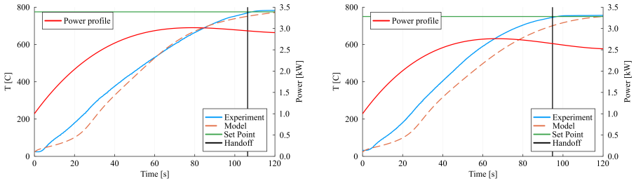
The central claim is that a first-law lumped-capacitance temperature model, in which the unknown conversion factor from machine power to internal heating is replaced by a small sigmoid-output neural network, can be fitted by gradient descent through an ODE solver and then used, with weights frozen, to design open-loop control inputs that achieve set-point temperatures on an actual friction-stir processing machine. The control input is constrained to the third-order polynomial power profile the machine's built-in controller expects, with the constant term fixed at the measured idle power draw. Across two validation batches, all six runs reached final handoff temperatures at or below 1% of the 750 or 775 degree Celsius setpoints. Mean absolute percent errors of roughly 7 to 20 percent during the plunge are dominated by a time lag in the first about 20 seconds after tool contact, and the authors note that model and experiment align after that. The result is offered as validation that interpretable, data-enabled system dynamics models can carry out real-world process control tasks.
Load-bearing premise
The load-bearing assumption is that the machine's internal power controller delivers the commanded cubic power profile to the workpiece accurately enough that the model input matches the physics; the paper reports no direct measurement of delivered power or tracking error.
Editorial extensions
If this is right
- All six validation experiments reached handoff within 1% of setpoint, including two setpoints absent from the training data, so the method transfers to unseen setpoints without manual retuning.
- Changing a single smoothing hyperparameter produced distinct fast and slow profiles to the same setpoint, indicating the framework can shape time-to-temperature.
- The differentiable model plus trajectory optimization gives a direct path to closed-loop feedback control once hardware supports real-time sampling and control.
- The same system identification pipeline should apply to other alloys and processing conditions by retraining or fine-tuning the neural conversion factor.
Reading between the lines
- The 1% end-state criterion is what is validated; the paper's own error metrics show the model is not yet accurate about the early transient, so any claim about defect formation during the first seconds of plunge is not established.
- Because delivered power is never measured, the neural network may have implicitly absorbed the machine's internal controller behavior; the optimized profiles may need re-validation on a machine with different power-tracking characteristics.
- A direct next experiment would be to rerun one of the validated profiles after intentionally changing the machine's power-controller gains; if handoff accuracy persists, the model is robust to actuator details, and if not, the controller tracking is the true load-bearing element.
Signed reviews
Editorial analysis
A structured set of objections, weighed in public.
Referee Report
Summary. The manuscript proposes and experimentally tests an open-loop, model-based controller for the plunge phase of friction-stir processing (FSP). The authors train a neural lumped-parameter ODE (Eq. 1) on temperature time series from seven FSP runs, then freeze that model and optimize the coefficients of a cubic power profile (Eq. 4) to drive the modeled tool temperature to a desired setpoint while penalizing energy, roughness, and overshoot. The optimized profiles are loaded into the machine's built-in power controller and evaluated in six experiments at two setpoints (750 and 775 °C). The paper reports that the measured tool temperature at the power-to-temperature handoff was within 1% of setpoint in all six runs.
Significance. If the claimed results are robust, this is a worthwhile proof-of-concept: it demonstrates that a physically structured data-driven model can generate open-loop power profiles for FSP without manual tuning, and the method is transparent and inexpensive to train. The clarity of the model description and the use of standard, reproducible numerical tools (Julia's DifferentialEquations.jl and DiffEqFlux.jl) are strengths. However, the validation is currently too limited to establish the general capability claimed in the title and abstract.
major comments (4)
- [§2.4, with Figs. 2b and 4-9] The controller commands a polynomial power profile to the machine's internal PID, but the model in Eq. (1) was trained on realized power ("given actual power input," Fig. 2b). The paper does not report the actual power delivered during the six validation runs, nor the PID tracking error, spindle speed, or torque. If the realized power deviates from the commanded cubic profile (e.g., due to PID lag or the 1 kW idle offset), the measured temperature trajectories cannot be attributed to the model-generated profile. Please provide measured power (or acceptable proxies) and quantify tracking error; if these data are unavailable, the central claim must be explicitly limited to commanded, not delivered, power.
- [§3.1-3.2] The validation is thin: only two previously unseen setpoints (775 and 750 °C) appear in Batch 1, and Batch 2 repeats those same two setpoints with different speed profiles. Each condition was run once, so there are no error bars or repeated trials, and no baseline comparison (e.g., hand-tuned linear ramps or the machine's default temperature control) is reported. The "within 1%" claim therefore rests on single measurements per condition. I ask for at least three repetitions per condition and a comparison to a standard or manual baseline to support the claim that the data-driven profiles provide value.
- [Eq. (3), L_smoothing] The smoothing penalty is defined as a sum of first differences P(t^{k+1}) - P(t^k) without an absolute value or a square. As written, this term can be negative and does not penalize roughness as the text claims; it would instead reward a monotonically decreasing profile. Please correct the equation (likely |ΔP| or (ΔP)^2) and confirm what was actually implemented in the optimization, since the loss is load-bearing for the reported control profiles.
- [§3, handoff metric] The primary performance metric is the temperature at the moment the machine automatically switches from power control to temperature control. Because the switch is triggered by reaching the setpoint, the "handoff temperature" is partly determined by the machine's own threshold logic, which makes the "within 1%" claim less informative than a metric like time-to-setpoint, overshoot, or the full temperature trajectory error. The paper reports Max T in Table 1, but it should explicitly report the time-to-handoff and overshoot for each run, and the model-experiment error over the entire plunge, not only at the handoff.
minor comments (6)
- [§4] The term "model predictive control" is used to describe the offline trajectory optimization of Section 2.3, but true MPC employs closed-loop receding-horizon feedback; please use "open-loop optimal control" or "trajectory optimization" to avoid confusion.
- [Eq. (3)] The overshoot term uses relu but does not define it; please define relu(x)=max(0,x).
- [Table 1] The meaning of "Max T" is unclear (maximum temperature during the plunge, after handoff, or including the traverse?); please define it in the caption.
- [§2.2] "an scheme" should be "a scheme".
- [§2.2-2.3] The paper does not report the number of data points per experimental run or the time step used in the ODE solver; please add these details for reproducibility.
- [Table 1] The MAPE values up to 20.5% are attributed to time delays in the initial contact phase; a brief discussion of whether these delays arise from PID tracking error or from model error would help the reader assess the controller's robustness.
Circularity Check
No circularity: the control profiles are optimized against a fitted model, and the validation is an independent hardware test on setpoints outside the training distribution in Batch #1.
full rationale
The central derivation chain is system identification (Eq. 2) followed by open-loop trajectory optimization (Eq. 3) and hardware validation. The model is fitted to temperature time series from hand-tuned linear power profiles; the control optimization then freezes the fitted parameters and minimizes a setpoint loss with respect to the polynomial power coefficients. The resulting profile is deployed on the FSP machine. The final handoff temperatures are experimental measurements, not quantities recovered from the optimization objective, so the within-1% claim is not equivalent to the training objective by construction. Batch #1 explicitly targets setpoints (775C and 750C) that were absent from the training data, making the hardware test an extrapolation. Batch #2 retrains on the added Batch #1 data, but the new fast/slow profiles are distinct control inputs, so the validation still tests the model on new inputs. The only citation to prior work by the same authors, Ref. [4], supplies the model form and dataset details, but the system ID and control optimizations are re-run in the present paper, so the citation is not load-bearing circularity. A genuine limitation is that the machine's internal PID tracking of the commanded cubic profile is not measured, so realized power is assumed to equal commanded power; this is an experimental-validation gap (correctness risk), not a circularity. No step reduces to its own inputs by definition.
Assumptions & free parameters
free parameters (4)
- Thermal capacitance C =
not reported
- Heat transfer coefficient h =
not reported
- Neural network weights θ =
not reported (61 weights for a 2-15-1 MLP)
- Loss hyperparameters λ1-4 =
(1, 1e3, 1e6, 1e3) fast; (1, 1e3, 1e7, 1e3) slow
assumptions (7)
- standard math First Law of Thermodynamics energy balance
- domain assumption Lumped capacitance with uniform temperature
- domain assumption Linear heat transfer to a constant sink
- ad hoc to paper Neural network η(T,P) with sigmoid output in (0,1) can represent the true power conversion efficiency
- ad hoc to paper Power profile restricted to a third-order polynomial
- domain assumption The machine's PID controller tracks commanded power
- domain assumption Thermocouple temperature in tool shoulder is the controlled temperature
Cite this review
Pith. "Pith review of First Contact: Data-driven Friction-Stir Process Control." pith.science (2026). https://pith.science/paper/3A6IPXO6
@misc{pith2026250703177,
  author       = {Pith},
  title        = {Pith review of: First Contact: Data-driven Friction-Stir Process Control},
  year         = {2026},
  howpublished = {\url{https://pith.science/paper/3A6IPXO6}},
  note         = {Machine review of arXiv:2507.03177}
}
read the original abstract
This study validates the use of Neural Lumped Parameter Differential Equations for open-loop setpoint control of the plunge sequence in Friction Stir Processing (FSP). The approach integrates a data-driven framework with classical heat transfer techniques to predict tool temperatures, informing control strategies. By utilizing a trained Neural Lumped Parameter Differential Equation model, we translate theoretical predictions into practical set-point control, facilitating rapid attainment of desired tool temperatures and ensuring consistent thermomechanical states during FSP. This study covers the design, implementation, and experimental validation of our control approach, establishing a foundation for efficient, adaptive FSP operations.
Figures


Figures from the paper (3 more)


Reference graph
Works this paper leans on
-
[1]
write newline
" write newline "" before.all 'output.state := FUNCTION n.dashify 't := "" t empty not t #1 #1 substring "-" = t #1 #2 substring "--" = not "--" * t #2 global.max substring 't := t #1 #1 substring "-" = "-" * t #2 global.max substring 't := while if t #1 #1 substring * t #2 global.max substring 't := if while FUNCTION word.in bbl.in ":" * " " * FUNCTION f...
-
[2]
write newline
" write newline "" before.all 'output.state := FUNCTION n.dashify 't := "" t empty not t #1 #1 substring "-" = t #1 #2 substring "--" = not "--" * t #2 global.max substring 't := t #1 #1 substring "-" = "-" * t #2 global.max substring 't := while if t #1 #1 substring * t #2 global.max substring 't := if while FUNCTION word.in bbl.in ":" * " " * FUNCTION f...
-
[3]
write newline
" write newline "" before.all 'output.state := FUNCTION n.dashify 't := "" t empty not t #1 #1 substring "-" = t #1 #2 substring "--" = not "--" * t #2 global.max substring 't := t #1 #1 substring "-" = "-" * t #2 global.max substring 't := while if t #1 #1 substring * t #2 global.max substring 't := if while FUNCTION word.in bbl.in ":" * " " * FUNCTION f...
-
[4]
R. S. Mishra, Z. Ma, Friction stir welding and processing, Materials science and engineering: R: reports 50 (1-2) (2005) 1--78
work page 2005
-
[5]
A. Heidarzadeh, S. Mironov, R. Kaibyshev, G. C am, A. Simar, A. Gerlich, F. Khodabakhshi, A. Mostafaei, D. P. Field, J. D. Robson, et al., Friction stir welding/processing of metals and alloys: a comprehensive review on microstructural evolution, Progress in Materials Science 117 (2021) 100752
work page 2021
-
[6]
P. Kah, R. Rajan, J. Martikainen, R. Suoranta, Investigation of weld defects in friction-stir welding and fusion welding of aluminium alloys, International Journal of Mechanical and Materials Engineering 10 (2015) 1--10
work page 2015
-
[7]
J. Koch, W. Choi, E. King, D. Garcia, H. Das, T. Wang, K. Ross, K. Kappagantula, Neural lumped parameter differential equations with application in friction-stir processing, Journal of Intelligent Manufacturing (2024) 1--11
work page 2024
-
[8]
C. Rackauckas, Y. Ma, J. Martensen, C. Warner, K. Zubov, R. Supekar, D. Skinner, A. Ramadhan, A. Edelman, Universal differential equations for scientific machine learning, arXiv preprint arXiv:2001.04385 (2020)
arXiv 2020
Show all 11 references
-
[9]
R. T. Chen, Y. Rubanova, J. Bettencourt, D. K. Duvenaud, Neural ordinary differential equations, Advances in neural information processing systems 31 (2018)
2018
-
[10]
Drgo n a, K
J. Drgo n a, K. Ki s , A. Tuor, D. Vrabie, M. Klau c o, Differentiable predictive control: Deep learning alternative to explicit model predictive control for unknown nonlinear systems, Journal of Process Control 116 (2022) 80--92
2022
-
[11]
Rackauckas, Q
C. Rackauckas, Q. Nie, Differentialequations.jl--a performant and feature-rich ecosystem for solving differential equations in julia, Journal of Open Research Software 5 (1) (2017)
2017
Reviewed August 6, 2026 · model on record in the stance chip above.
Discussion (0). Continue with ORCID to comment.