REVIEW 5 major objections 5 minor 56 references
PINN-DG: Residual neural network methods trained with Finite Elements
T0 review · 5 major / 5 minor · reviewed 2026-08-06 · deepseek-v4-flash
Pith's one-line read A discontinuous-Galerkin finite element loss for PINNs is proven to converge to the exact solution of Poisson's equation as the mesh and network refine in step.
desk verdict Genuinely useful FE-interpolated PINN training with DG stabilization, but the convergence proof has a repairable gap in Lemma 3.3 and sign errors that need fixing. read the letter →
The pith
A machine-rendered reading of the paper's core claim, the machinery that carries it, and where it could break.
The reading
What carries the argument
The load-bearing object is the DG-interpolated residual energy (3.1): $$E_\ell(u_\ell) = \sum_{K\in T_h} \int_K |\$\Delta$ I_S u_\ell + I_S f|^2\,dx - 2\sum_{e\in E^i_h} \int_e \{\!\{\$\Delta$ I_S u_\ell + I_S f\}\!\} [\![\nabla I_S u_\ell \cdot n]!]\,ds + \$\alpha$\,\text{pen}(u_\ell),$$ with $I_S$ the $C^0$ Lagrangian interpolant into piecewise polynomials of degree $q\ge2$, $\{\!\{\cdot\}\!\}$ the average, $[\![\cdot]!]$ the jump across interior edges, and $\text{pen}(u_\ell)$ the inverse-mesh-weighted jumps of gradients plus a boundary penalty realizing Dirichlet conditions in the spirit of Nitsche's method. Rewriting via the lifting operator $R_h$, the energy is $\int_\Omega |L_h(u_{h,\ell})+f_h|^2 - |R_h(\nabla u_{h,\ell})|^2 + \alpha\,\text{pen}(u_\ell)$, where $L_h = \Delta_h - R_h(\nabla u_h)$ is a discrete Laplacian. This object simultaneously removes pointwise network second derivatives — the loss is assembled from finite element integrals — and supplies the coercivity and compactness needed for the $\Gamma$-convergence (lim inf–lim sup) proof: the lifting is $L^2$-bounded by the penalty, the discrete Laplacian passes weak limits to the true Laplacian (Lemma 3.1), and the consistency and jump terms vanish on recovery sequences.
What would settle it
Run the unit-square experiment of Section 4.1 with the four-block residual network, fix a mesh schedule satisfying $h(\ell)=c\beta_\ell$, and record the $L^2$ error of the interpolated minimizers as the loss decreases; if the errors fail to approach zero while the discrete losses do, Theorem 3.1's convergence conclusion is not realized for that architecture, isolating either the approximation-rate premise or the scaling condition as the failing ingredient.
Extended reading notes
Core claim
The central claim is that replacing the pointwise residual loss of a PINN with a discontinuous-Galerkin finite element loss does not sacrifice consistency: minimizers $u_\ell$ of the discrete energy $E_\ell$ converge, after $C^0$ finite element interpolation, weakly in $H^1$ and strongly in $L^2$ to the unique minimizer $u$ of the continuous residual energy $\int_\Omega |\Delta u + f|^2\,dx$, provided $h(\ell) = c\beta_\ell$ for a constant $c>0$ and the boundary-mesh condition $h_{E,\ell}^{-1/2}(\tilde\beta_\ell^{[2,0,\infty]})^{1-2\epsilon} \le C$ holds, where $\beta_\ell$ is the best network approximation rate from (2.18). Since the unique minimizer of $E$ is the weak solution of Poisson's equation, the theorem states that the DG-trained networks approximate the PDE solution in the limit.
Load-bearing premise
The load-bearing premise is that the neural network spaces actually contain functions that approximate the exact solution to the steadily improving degrees described in assumption (2.18), and that the mesh is refined in step with those rates; if the optimizer does not find such approximants, the $\Gamma$-convergence proof does not apply.
Editorial extensions
If this is right
- For elliptic problems like Poisson's equation, training a PINN can be performed entirely through finite element assembly and quadrature, eliminating automatic differentiation of the network's second derivative in the loss.
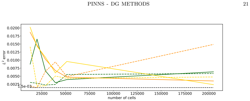
- The gradient-jump consistency terms carry the stability: without them, deeper residual networks show $L^2$ errors one to two orders of magnitude larger even as the reported loss decreases.
- Weak imposition of Dirichlet data through the boundary penalty means the network architecture does not need to encode boundary conditions.
- Any accumulation point of the interpolated discrete minimizers is the exact solution of the Poisson problem, so the convergence conclusion is independent of optimizer-specific behaviour once the approximation-rate hypothesis holds.
- On nonconvex domains with corner singularities the FE-trained method still converges under refinement, with $L^2$ error decreasing from about $6\cdot10^{-2}$ to $9\cdot10^{-3}$ in the reported L-shaped test.
Reading between the lines
- The same DG-interpolation template should transfer to other second-order elliptic operators and to nonlinear least-squares residual energies whenever a coercive DG discretisation with a bounded lifting exists, since the proof mechanism is not specific to the Poisson operator.
- The scaling condition $h(\ell)=c\beta_\ell$ could be turned into an adaptive algorithm: estimate the network's approximation rate during training and refine the mesh accordingly, and the theorem predicts a convergent schedule.
- The jump-free failure mode suggests that pure residual PINN losses can be fooled by nearly discontinuous functions that quadrature misses, so adding a DG-style jump penalty to collocation-based PINNs may improve robustness, although the paper does not test this.
- Extending to parabolic or hyperbolic problems would require a time-discrete version of the discrete Laplacian; the variational template indicates a route, but new coercivity and compactness estimates for the evolution operator would be needed.
Editorial analysis
A structured set of objections, weighed in public.
Referee Report
Summary. The paper introduces PINN-DG, a physics-informed neural network method for elliptic boundary value problems in which the network is interpolated into a C0 finite element space and a discontinuous-Galerkin-type discrete energy, including gradient jump consistency terms and a Nitsche-style penalty, is minimized. The central theoretical claim is a Gamma-convergence result: under an abstract neural-network approximation property and the scaling h(ell)=c beta_ell, minimizers of the discrete energy, after finite element interpolation, converge weakly in H1 and strongly in L2 to the unique minimizer of the continuous residual energy, which solves Poisson's equation. The paper also reports numerical experiments on square and L-shaped domains showing accuracy, robustness for deeper networks, and computational and memory savings relative to collocation-based PINNs. The main proof is built on an equicoercivity proposition and a lim inf / lim sup Gamma-convergence argument.
Significance. If completed, the paper gives a useful convergence framework for a practical hybrid method: replacing pointwise network derivatives with finite element interpolation and DG jump terms is a genuinely attractive way to reduce cost and memory in residual-based PINN training. The conditional structure of the theorem, based on abstract network approximation rates, is clearly stated and is compatible with standard neural-network approximation results. The numerical experiments support the practical value of the method, particularly the stabilizing role of the jump terms for deeper networks. However, the theoretical proof as printed has a load-bearing gap in the lim sup lemma, as well as several sign and regularity inconsistencies, so the central convergence claim is not fully established in the current version.
major comments (5)
- [§3.4, Lemma 3.3, Eq. (3.27)] The proof of the lim sup inequality is incomplete. The lemma's goal (3.27) contains two limits, but the estimates (3.28)-(3.35) address only the first: they bound the difference between ||Δw_{ell,delta}+f_ell||^2_{L2} and E_ell(w_{ell,delta}) and show that the consistency and penalty terms vanish. There is no argument establishing the second limit, ||Δw_{ell,delta}+f_ell||^2_{L2} -> E(w), along the diagonal delta=h(ell)^{1/4}, h(ell)=c beta_ell. A triangle-inequality estimate such as | ||Δw_{ell,delta}+f_ell||^2_{L2} - E(w) | <= C( beta_ell^{[3,2,2]} delta^{-2} + ||f_ell-f||_{L2} + delta ) would supply the missing step. Without it the recovery sequence is not shown to satisfy the lim sup inequality, and Theorem 3.1 is not fully established.
- [§3.4, Theorem 3.1 and Lemma 3.3, Eqs. (3.30)-(3.32)] The rates used in Lemma 3.3 are not controlled by the rates assumed in Theorem 3.1. The proof of (3.30)-(3.32) requires the approximation rate beta_ell^{[4,3,2]} appearing in (3.26) with s=4, i.e. ||w_{ell,delta}-w_delta||_{H^3} <= beta_ell^{[4,3,2]} |w_delta|_{H^4}. The definition of beta_ell in Theorem 3.1 is the maximum of beta_ell^{[1,0,2]}, beta_ell^{[2,1,2]}, beta_ell^{[3,2,2]}, and beta_ell^{[4,2,2]} only. Therefore the proof uses a rate that is not an assumption of the theorem; either beta_ell must be enlarged to include beta_ell^{[4,3,2]}, or the estimates in Lemma 3.3 must be reworked so that only the listed rates are used.
- [§3.4, Lemma 3.2, Eq. (3.24)] Equation (3.24) rewrites E_ell(v_ell) as ||L_{h(ell)}(bv_ell)+f_ell||^2_{L2} + ||R_h(∇bv_ell)||^2_{L2} + alpha pen(v_ell), but the definition in (3.6) contains -||R_h(∇bv_ell)||^2_{L2}. The subsequent inequality in (3.24) effectively uses the correct negative sign together with the lifting bound (3.8), but the displayed identity is wrong and must be corrected. The same issue occurs in the integration-by-parts identity (3.19), where the volume term sum_K ∫_K bv_ell Δbv_ell should carry a minus sign; the proof is insensitive to this because it estimates absolute values, but the identity as printed is incorrect.
- [§3.4, Theorem 3.1, boundary-mesh condition] The assumption h_{E,ell}^{-1/2} (beta_ell^{[2,0,∞]})^{1-2ε} <= C stated in Theorem 3.1 is never used in the proof. The boundary penalty estimate (3.33)-(3.35) is performed entirely with h(ell) and the rates beta_ell^{[1,0,2]} and beta_ell^{[2,1,2]}; no lower bound on boundary edge lengths or the parameter ε appears. Either the proof should show where this condition is needed, or the condition should be removed, since an unused hypothesis makes the convergence statement unnecessarily restrictive and unverifiable in the experiments.
- [§2.1, Proposition 2.1, Eq. (2.10)] The proof of estimate (2.9) contains an unjustified step. In (2.10), the bound (∑_{e∈E^i_h} h_e^{-1} ||f_h||^2_{L^2(K_e)})^{1/2} ≲ ||f_h||_{L^2(Ω)} is asserted, but for a generic piecewise polynomial f_h, already for f constant on a uniform mesh, the left-hand side is of order h^{-1/2}||f_h||, not bounded by a constant times ||f_h||. The statement of Proposition 2.1 also does not state the regularity of f, while the proof uses f ∈ C^0(Ω) and then invokes ||f||_{H^1(Ω)}. Since Lemma 3.3 uses (2.9) to show the consistency term vanishes, this estimate, or its hypotheses, must be repaired.
minor comments (5)
- [Proof of Theorem 3.1] The bound ||ũ - bu_ell||_{L^2(∂Ω)} ≲ ||ũ - bu_ell||_{L^2(Ω)} ||ũ - bu_ell||_{H^1(Ω)} is not the standard multiplicative trace inequality, which has square roots on the two norms; the conclusion is unaffected because both factors tend to zero, but the displayed estimate should be corrected.
- [§3.2, Lemma 3.1, Eq. (3.13)] In the chain of estimates (3.13), the constant factors from the uniform bound (3.10) are omitted, and the second term should carry the factor (∑_e h_e^{-1} ||J∇u_h K||^2)^{1/2}; as printed, an independent factor h |φ|_{H^1} appears without explanation.
- [§3.4, Lemma 3.3, Eq. (3.32)] The simplification h(ell)^2 δ^{-4} ( (beta_ell^{[4,3,2]})^2 δ^{-2} + 1 ) = h(ell) + h(ell)^{3/4} is not consistent with the substitution h(ell) = beta_ell and δ = h(ell)^{1/4}; the correct leading terms are of orders h^{5/2} and h. Since both tend to zero, this is cosmetic but should be fixed.
- [Proof of Theorem 3.1, Eq. (3.36)] The notation j_ell(ũ_ell) + b_ell(ũ_ell) in (3.36) is undefined; it should refer to the internal-edge and boundary parts of pen(u_ell), respectively.
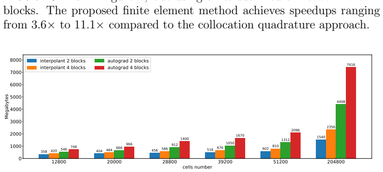
- [§4, Computational Experiments] The numerical experiments report speedups and memory comparisons but do not state the number of independent runs or any error bars; adding this information would strengthen the robustness claims.
Circularity Check
No circularity: the convergence theorem is a conditional Gamma-convergence argument with explicit approximation assumptions; the authors' self-citations are contextual and not load-bearing.
full rationale
The paper's central derivation is self-contained in the sense required by the circularity test: no quantity is defined in terms of the result being proved, no parameter is fitted to data and then renamed as a prediction, and the convergence theorem rests on explicitly stated assumptions rather than on a self-citation chain. The discrete loss (3.7) is constructed from finite element interpolation, DG consistency terms, and penalty terms; Theorem 3.1 then proves convergence of its minimizers under the abstract neural-network approximation assumption (2.18) and the scaling h(ell) = c beta_ell together with the stated boundary-mesh condition. These hypotheses are declared as assumptions in the text ('we now describe the approximation properties of neural network spaces. For each ell in N... there exists w_ell in V_ell satisfying (2.18)'), and they are not derived from the theorem's conclusion. Lemma 3.2 and Lemma 3.3 use standard Gamma-convergence estimates; technical support is drawn from external references such as Di Pietro-Ern, Buffa-Ortner, and Brenner-Scott, alongside the authors' prior work [24], [27], [29]. The self-citations situate the method within the authors' earlier frameworks, but the proof of Theorem 3.1 is re-derived rather than imported wholesale: Lemma 3.1 is proved in the text, Proposition 3.1 is proved in the text, and Lemma 3.3 supplies its own estimates. The only notable manuscript-level issue is a completeness gap, not circularity: in Lemma 3.3 the second limit in (3.27), namely |E(w) - ||Delta w_{ell,delta} + f_ell||^2_{L2}| -> 0, is asserted but not explicitly estimated; this is a missing proof step that would need to be supplied for the lim sup inequality to be fully rigorous as written. That is a correctness risk, not a reduction of the result to its inputs. Accordingly, no circular step is exhibited and the circularity score is 0.
Assumptions & free parameters
free parameters (2)
- Penalty parameter alpha =
60 in experiments; alpha > C_R in theory
- Scaling constant c in h(ell) = c beta_ell =
unspecified
assumptions (5)
- domain assumption Abstract neural network approximation property (2.18): for each ell there exists w_ell in V_ell approximating w in W^{s,p} with rate beta_ell tending to zero.
- standard math C0 Lagrange interpolation estimates (2.6) and trace estimates (2.7) hold on shape-regular triangulations.
- standard math The DG lifting operator R_h satisfies the L2 bound (3.8) from [13, 19].
- ad hoc to paper Scaling condition h(ell) = c beta_ell and boundary-mesh condition h^{-1/2}_{E,ell} (beta_tilde[2,0,infty])^{1-2epsilon} <= C in Theorem 3.1.
- domain assumption Elliptic regularity and smooth approximation of V functions with zero boundary data, as described in Remark 3.1.
Cite this review
Pith. "Pith review of PINN-DG: Residual neural network methods trained with Finite Elements." pith.science (2026). https://pith.science/paper/WIW2LS2U
@misc{pith2026250703521,
  author       = {Pith},
  title        = {Pith review of: PINN-DG: Residual neural network methods trained with Finite Elements},
  year         = {2026},
  howpublished = {\url{https://pith.science/paper/WIW2LS2U}},
  note         = {Machine review of arXiv:2507.03521}
}
read the original abstract
Over the past few years, neural network methods have evolved in various directions for approximating partial differential equations (PDEs). A promising new development is the integration of neural networks with classical numerical techniques such as finite elements and finite differences. In this paper, we introduce a new class of Physics-Informed Neural Networks (PINNs) trained using discontinuous Galerkin finite element methods. Unlike standard collocation-based PINNs that rely on pointwise gradient evaluations and Monte Carlo quadrature, our approach computes the loss functional using finite element interpolation and integration. This avoids costly pointwise derivative computations, particularly advantageous for elliptic PDEs requiring second-order derivatives, and inherits key stability and accuracy benefits from the finite element framework. We present a convergence analysis based on variational arguments and support our theoretical findings with numerical experiments that demonstrate improved efficiency and robustness.
Figures


Figures from the paper (7 more)




Reference graph
Works this paper leans on
-
[1]
G. Akrivis, C. G. Makridakis, and C. Smaragdakis. Runge-Kutta Physics Informed Neural Networks: Formulation and Analysis. 2025. arXiv: 2412.20575 [math.NA]. url: https://arxiv.org/abs/2412.20575
arXiv 2025
-
[2]
Finite element interpolated neural net- works for solving forward and inverse problems
S. Badia, W. Li, and A. F. Mart´i n. “Finite element interpolated neural net- works for solving forward and inverse problems”. Computer Methods in Applied Mechanics and Engineering 418 (Jan. 2024), p. 116505. url: http://dx.doi. org/10.1016/j.cma.2023.116505
-
[3]
Physics Informed Neural Networks (PINNs)for approximating nonlinear dispersive PDEs
G. Bai, U. Koley, S. Mishra, and R. Molinaro. “Physics informed neural net- works (PINNs) for approximating nonlinear dispersive PDEs”. arXiv preprint arXiv:2104.05584 (2021)
work page Pith review arXiv 2021
-
[4]
Physics informed neural networks (PINNs) for approximating nonlinear dispersive PDEs
G. Bai, U. Koley, S. Mishra, and R. Molinaro. “Physics informed neural networks (PINNs) for approximating nonlinear dispersive PDEs”. J. Comput. Math. 39.6 (2021), pp. 816–847. url: https://doi.org/10.4208/jcm.2101-m2020-0342
-
[5]
S. Bartels, A. Bonito, and R. H. Nochetto. “Bilayer Plates: Model Reduction, Γ- Convergent Finite Element Approximation, and Discrete Gradient Flow”. Com- munications on Pure and Applied Mathematics 70.3 (2017), pp. 547–589
work page 2017
-
[6]
J. Berg and K. Nystr¨ om. “A unified deep artificial neural network approach to partial differential equations in complex geometries”. Neurocomputing 317 (Nov. 2018), pp. 28–41. url: https://doi.org/10.1016%2Fj.neucom.2018.06.056
work page 2018
-
[7]
The modern mathematics of deep learning
J. Berner, P. Grohs, G. Kutyniok, and P. Petersen. “The modern mathematics of deep learning”. Mathematical aspects of deep learning. Cambridge Univ. Press, Cambridge, 2023, pp. 1–111
work page 2023
-
[8]
Variational physics informed neural net- works: the role of quadratures and test functions
S. Berrone, C. Canuto, and M. Pintore. “Variational physics informed neural net- works: the role of quadratures and test functions”. J. Sci. Comput. 92.3 (2022), Paper No. 100, 27. url: https://doi.org/10.1007/s10915-022-01950-4
Show all 56 references
-
[9]
C 0 interior penalty methods for fourth order elliptic boundary value problems on polygonal domains
S. C. Brenner and L.-Y. Sung. “C 0 interior penalty methods for fourth order elliptic boundary value problems on polygonal domains”. Journal of Scientific Computing 22.1 (2005), pp. 83–118
2005
-
[10]
S. C. Brenner and L. R. Scott. The mathematical theory of finite element meth- ods. Third. Vol. 15. Texts in Applied Mathematics. Springer, New York, 2008, pp. xviii+397. url: https://doi.org/10.1007/978-0-387-75934-0
2008 doi
-
[11]
H. Brezis. Functional analysis, Sobolev spaces and partial differential equations . Springer Science & Business Media, 2010. REFERENCES 27
2010
-
[12]
Discontinuous Galerkin approximations for elliptic problems
F. Brezzi, G. Manzini, D. Marini, P. Pietra, and A. Russo. “Discontinuous Galerkin approximations for elliptic problems”. Numerical Methods for Partial Differential Equations: An International Journal 16.4 (2000), pp. 365–378
2000
-
[13]
Compact embeddings of broken Sobolev spaces and applications
A. Buffa and C. Ortner. “Compact embeddings of broken Sobolev spaces and applications”. IMA journal of numerical analysis 29.4 (2009), pp. 827–855
2009
-
[14]
A Deep Learning Approach to Non- convex Energy Minimization for Martensitic Phase Transitions
X. Chen, P. Rosakis, Z. Wu, and Z. Zhang. “A Deep Learning Approach to Non- convex Energy Minimization for Martensitic Phase Transitions”. arXiv preprint 2206.13937 (2022). arXiv: 2206.13937 [cs.CE]
2022 arXiv
-
[15]
CA special issue on neural network approximation
W. Dahmen, R. A. DeVore, and P. Grohs. “CA special issue on neural network approximation”. Constr. Approx. 55.1 (2022), pp. 1–2. url: https://doi.org/ 10.1007/s00365-021-09547-0
2022 doi
-
[16]
De Giorgi
E. De Giorgi. Selected papers. Springer Collected Works in Mathematics. [Author name on title page: Ennio Giorgi], Edited by Luigi Ambrosio, Gianni Dal Maso, Marco Forti, Mario Miranda and Sergio Spagnolo, Reprint of the 2006 edition [MR2229237]. Springer, Heidelberg, 2013, pp. x+888
2006
-
[17]
On the approximation of rough functions with deep neural networks
T. De Ryck, S. Mishra, and D. Ray. “On the approximation of rough functions with deep neural networks”. SeMA J. 79.3 (2022), pp. 399–440. url: https : //doi.org/10.1007/s40324-022-00299-w
2022 doi
-
[18]
Discrete functional analysis tools for discontinuous Galerkin methods with application to the incompressible Navier-Stokes equa- tions
D. Di Pietro and A. Ern. “Discrete functional analysis tools for discontinuous Galerkin methods with application to the incompressible Navier-Stokes equa- tions”. Mathematics of Computation 79.271 (2010), pp. 1303–1330
2010
-
[19]
D. A. Di Pietro and A. Ern. Mathematical aspects of discontinuous Galerkin meth- ods. Vol. 69. Springer Science & Business Media, 2011
2011
-
[20]
The deep Ritz method: a deep learning-based numerical al- gorithm for solving variational problems
W. E and B. Yu. “The deep Ritz method: a deep learning-based numerical al- gorithm for solving variational problems”. Communications in Mathematics and Statistics 6.1 (2018), pp. 1–12
2018
-
[21]
Engel, K
G. Engel, K. Garikipati, T. J. Hughes, M. G. Larson, L. Mazzei, and R. L. Taylor. “Continuous/discontinuous finite element approximations of fourth-order elliptic problems in structural and continuum mechanics with applications to thin beams and plates, and strain gradient ela...
2002
-
[22]
L. C. Evans. Partial Differential Equations. Vol. 19. American Mathematical Soc., 2010. 28 REFERENCES
2010
-
[23]
A High-Efficient Hybrid Physics-Informed Neural Networks Based on Convolutional Neural Network
Z. Fang. “A High-Efficient Hybrid Physics-Informed Neural Networks Based on Convolutional Neural Network”.IEEE Transactions on Neural Networks and Learn- ing Systems 33.10 (2022), pp. 5514–5526
2022
-
[24]
Gazoulis, I
D. Gazoulis, I. Gkanis, and C. G. Makridakis. On the Stability and Convergence of Physics Informed Neural Networks . arXiv2308.05423. 2023. arXiv: 2308.05423 [math.NA]. url: https://arxiv.org/abs/2308.05423
2023 arXiv
-
[25]
Discrete gradient flow approxi- mations of high dimensional evolution partial differential equations via deep neural networks
E. H. Georgoulis, M. Loulakis, and A. Tsiourvas. “Discrete gradient flow approxi- mations of high dimensional evolution partial differential equations via deep neural networks”. Communications in Nonlinear Science and Numerical Simulation 117 (2023), p. 106893
2023
-
[26]
A class of discontinuous Galerkin methods for nonlinear variational problems
G. Grekas, K. Koumatos, C. Makridakis, and A. Vikelis. “A class of discontinuous Galerkin methods for nonlinear variational problems”. Mathematics of Computa- tion (Jan. 2025). url: http://dx.doi.org/10.1090/mcom/4040
2025 doi
-
[27]
Approximations of energy minimization in cell-induced phase transitions of fibrous biomaterials: Γ- convergence analysis
G. Grekas, K. Koumatos, C. Makridakis, and P. Rosakis. “Approximations of energy minimization in cell-induced phase transitions of fibrous biomaterials: Γ- convergence analysis”. SIAM J. Numer. Anal. 60.2 (2022), pp. 715–750
2022
-
[28]
Grekas, K
G. Grekas, K. Koumatos, C. Makridakis, and A. Vikelis. Convergence of Discontin- uous Galerkin Methods for Quasiconvex and Relaxed Variational Problems . 2025. arXiv: 2501.11944 [math.NA]. url: https://arxiv.org/abs/2501.11944
2025 arXiv
-
[29]
Deep Ritz - Finite element methods: Neural network methods trained with finite elements
G. Grekas and C. G. Makridakis. “Deep Ritz - Finite element methods: Neural network methods trained with finite elements”. Computer Methods in Applied Mechanics and Engineering 437 (Mar. 2025), p. 117798. url: http://dx.doi. org/10.1016/j.cma.2025.117798
2025
-
[30]
Space-time error es- timates for deep neural network approximations for differential equations
P. Grohs, F. Hornung, A. Jentzen, and P. Zimmermann. “Space-time error es- timates for deep neural network approximations for differential equations”. Adv. Comput. Math. 49.1 (2023), Paper No. 4, 78. url: https://doi.org/10.1007/ s10444-022-09970-2
2023
-
[31]
Constructive deep ReLU neural network approximation
L. Herrmann, J. A. A. Opschoor, and C. Schwab. “Constructive deep ReLU neural network approximation”. J. Sci. Comput. 90.2 (2022), Paper No. 75, 37. url: https://doi.org/10.1007/s10915-021-01718-2
2022 doi
-
[32]
Q. Hong, J. W. Siegel, and J. Xu. A Priori Analysis of Stable Neural Network Solutions to Numerical PDEs . 2022. arXiv: 2104.02903 [math.NA]
2022 arXiv
-
[33]
Solving inverse problems in physics by optimizing a discrete loss: Fast and accurate learning without neural networks
P. Karnakov, S. Litvinov, and P. Koumoutsakos. “Solving inverse problems in physics by optimizing a discrete loss: Fast and accurate learning without neural networks”. PNAS Nexus 3.1 (Dec. 2023). Ed. by D. Abbott. url: http://dx. doi.org/10.1093/pnasnexus/pgae005. REFERENCES 29
2023 doi
-
[34]
Kharazmi, Z
E. Kharazmi, Z. Zhang, and G. E. Karniadakis. Variational Physics-Informed Neural Networks For Solving Partial Differential Equations . 2019. arXiv: 1912. 00873 [cs.NE]
2019
-
[35]
Artificial neural networks for solving ordi- nary and partial differential equations
I. Lagaris, A. Likas, and D. Fotiadis. “Artificial neural networks for solving ordi- nary and partial differential equations”. IEEE Transactions on Neural Networks 9.5 (1998), pp. 987–1000. url: https://doi.org/10.1109%2F72.712178
1998
-
[36]
A new approach to generalisation error of ma- chine learning algorithms: Estimates and convergence
M. Loulakis and C. G. Makridakis. “A new approach to generalisation error of ma- chine learning algorithms: Estimates and convergence”.arXiv preprint 2306.13784 (2023). arXiv: 2306.13784 [stat.ML]
2023 arXiv
-
[37]
On atomistic-to-continuum cou- plings without ghost forces in three dimensions
C. Makridakis, D. Mitsoudis, and P. Rosakis. “On atomistic-to-continuum cou- plings without ghost forces in three dimensions”. Applied Mathematics Research eXpress 2014.1 (2014), pp. 87–113
2014
-
[38]
C. G. Makridakis, A. Pim, and T. Pryer. A Deep Uzawa-Lagrange Multiplier Approach for Boundary Conditions in PINNs and Deep Ritz Methods. 2024. arXiv: 2411.08702 [math.NA]. url: https://arxiv.org/abs/2411.08702
2024 arXiv
-
[39]
C. G. Makridakis, A. Pim, and T. Pryer. Deep Uzawa for PDE constrained opti- misation. 2024. arXiv: 2410.17359 [math.NA]. url: https://arxiv.org/abs/ 2410.17359
2024 arXiv
-
[40]
R. E. Meethal, B. Obst, M. Khalil, A. Ghantasala, A. Kodakkal, K.-U. Bletzinger, and R. W¨ uchner.Finite Element Method-enhanced Neural Network for Forward and Inverse Problems . 2022. arXiv: 2205.08321 [cs.CE]. url: https://arxiv. org/abs/2205.08321
2022 arXiv
-
[41]
Estimates on the generalization error of physics- informed neural networks for approximating a class of inverse problems for PDEs
S. Mishra and R. Molinaro. “Estimates on the generalization error of physics- informed neural networks for approximating a class of inverse problems for PDEs”. IMA J. Numer. Anal. 42.2 (2022), pp. 981–1022. url: https://doi.org/10. 1093/imanum/drab032
2022
-
[42]
Estimates on the generalization error of physics- informed neural networks for approximating PDEs
S. Mishra and R. Molinaro. “Estimates on the generalization error of physics- informed neural networks for approximating PDEs”. IMA J. Numer. Anal. 43.1 (2023), pp. 1–43. url: https://doi.org/10.1093/imanum/drab093
2023 doi
-
[43]
Deep Ritz revisited
J. M¨ uller and M. Zeinhofer. “Deep Ritz revisited”.arXiv preprint arXiv:1912.03937 (2019)
2019 arXiv
-
[44]
¨Uber ein Variationsprinzip zur L¨ osung von Dirichlet-Problemen bei Verwendung von Teilr¨ aumen, die keinen Randbedingungen unterworfen sind
J. Nitsche. “ ¨Uber ein Variationsprinzip zur L¨ osung von Dirichlet-Problemen bei Verwendung von Teilr¨ aumen, die keinen Randbedingungen unterworfen sind”.Ab- handlungen aus dem mathematischen Seminar der Universit¨ at Hamburg. Vol. 36
-
[45]
1971, pp
Springer. 1971, pp. 9–15. 30 REFERENCES
1971
-
[46]
Pytorch: An imperative style, high- performance deep learning library
A. Paszke, S. Gross, F. Massa, A. Lerer, J. Bradbury, G. Chanan, T. Killeen, Z. Lin, N. Gimelshein, L. Antiga, et al. “Pytorch: An imperative style, high- performance deep learning library”. Advances in neural information processing systems 32 (2019)
2019
-
[47]
Discontinuous Galerkin methods for the p-biharmonic equation from a discrete variational perspective
T. Pryer. “Discontinuous Galerkin methods for the p-biharmonic equation from a discrete variational perspective”. Electron. Trans. Numer. Anal. 41 (2014), pp. 328–349
2014
-
[48]
Physics-informed neural net- works: a deep learning framework for solving forward and inverse problems in- volving nonlinear partial differential equations
M. Raissi, P. Perdikaris, and G. E. Karniadakis. “Physics-informed neural net- works: a deep learning framework for solving forward and inverse problems in- volving nonlinear partial differential equations”. J. Comput. Phys. 378 (2019), pp. 686–707. url: https://doi.org/10.101...
2019 doi
-
[49]
Hidden physics models: Machine learning of nonlinear partial differential equations
M. Raissi and G. E. Karniadakis. “Hidden physics models: Machine learning of nonlinear partial differential equations”. J. Comput. Phys. 357 (Mar. 2018), pp. 125–141. url: https://doi.org/10.1016%2Fj.jcp.2017.11.039
2018
-
[50]
Discrete- vs. continuous-time nonlinear signal processing of Cu electrodissolution data
R. Rico-Martinez, K. Krischer, I. Kevrekidis, M. Kube, and J. Hudson. “Discrete- vs. continuous-time nonlinear signal processing of Cu electrodissolution data”. Chemical Engineering Communications 118.1 (1992), pp. 25–48
1992
-
[51]
Deep learning in high dimension: neural network expres- sion rates for analytic functions in L2(Rd, γd)
C. Schwab and J. Zech. “Deep learning in high dimension: neural network expres- sion rates for analytic functions in L2(Rd, γd)”. SIAM/ASA J. Uncertain. Quantif. 11.1 (2023), pp. 199–234. url: https://doi.org/10.1137/21M1462738
2023 doi
-
[52]
On the convergence of physics in- formed neural networks for linear second-order elliptic and parabolic type PDEs
Y. Shin, J. Darbon, and G. E. Karniadakis. “On the convergence of physics in- formed neural networks for linear second-order elliptic and parabolic type PDEs”. Commun. Comput. Phys. 28.5 (2020), pp. 2042–2074. url: https://doi.org/ 10.4208/cicp.oa-2020-0193
2020 doi
-
[53]
Error estimates of residual minimiza- tion using neural networks for linear PDEs
Y. Shin, Z. Zhang, and G. E. Karniadakis. “Error estimates of residual minimiza- tion using neural networks for linear PDEs”. arXiv preprint 2010.08019 (2020). arXiv: 2010.08019 [math.NA]
2020 arXiv
-
[54]
DGM: a deep learning algorithm for solving partial differential equations
J. Sirignano and K. Spiliopoulos. “DGM: a deep learning algorithm for solving partial differential equations”. J. Comput. Phys. 375 (2018), pp. 1339–1364. url: https://doi.org/10.1016/j.jcp.2018.08.029
2018 doi
-
[55]
Discontinuous Galerkin methods for non-linear elas- ticity
A. Ten Eyck and A. Lew. “Discontinuous Galerkin methods for non-linear elas- ticity”. International Journal for Numerical Methods in Engineering 67.9 (2006), pp. 1204–1243
2006
-
[56]
Finite neuron method and convergence analysis
J. Xu. “Finite neuron method and convergence analysis”. Commun. Comput. Phys. 28.5 (2020), pp. 1707–1745. url: https://doi.org/10.4208/cicp.oa- 2020-0191. REFERENCES 31 Computer, Electrical, Mathematical Sciences & Engineering Division, King Abdul- lah University of Science an...
2020 doi
Reviewed August 6, 2026 · model on record in the stance chip above.
Discussion (0). Continue with ORCID to comment.