REVIEW 3 major objections 6 minor 5 cited by
Constraining the axiverse with reionization
T0 review · 3 major / 6 minor · reviewed 2026-08-06 · deepseek-v4-flash
Pith's one-line read Up to 15% of explicit string-theory axion models disfavor high-temperature reheating.
desk verdict A careful, genuinely new application of the string axiverse to reionization, with the headline 10–15% exclusion fractions resting on an explicitly assumed but unverified orientifold existence condition. read the letter →
The pith
A machine-rendered reading of the paper's core claim, the machinery that carries it, and where it could break.
The reading
What carries the argument
The machinery is the freeze-in abundance formula for each axion, $F_a \simeq F_{\rm Prim}+F_{\rm Id}$, combined with the two-photon decay rate $\Gamma_{a\to\gamma\gamma}=m_a^3 g_{a\gamma\gamma}^2/(64\pi)$. The freeze-in fraction scales with $T_{\rm reh}\, g_{a\gamma\gamma}^2 m_a$, so higher reheating temperatures produce more axions; the decay temperature decides whether the injected energy lands in the redshift window that contributes to $\tau_{\rm highz}$. The comparison target is a Gaussian-process posterior on $\tau_{\rm highz}$ with a 95% CL upper limit of 0.108, derived from CMB polarization data in the companion analysis. This lets the authors test multi-axion models against a model-independent reionization history rather than a single parametrized reionization scenario.
What would settle it
Explicitly construct compatible orientifolds for a random subset of the sampled polytope triangulations and recompute the excluded fractions using only those that exist; if the 15%, 15%, and 10% figures change substantially, the central ensemble claim fails.
Extended reading notes
Core claim
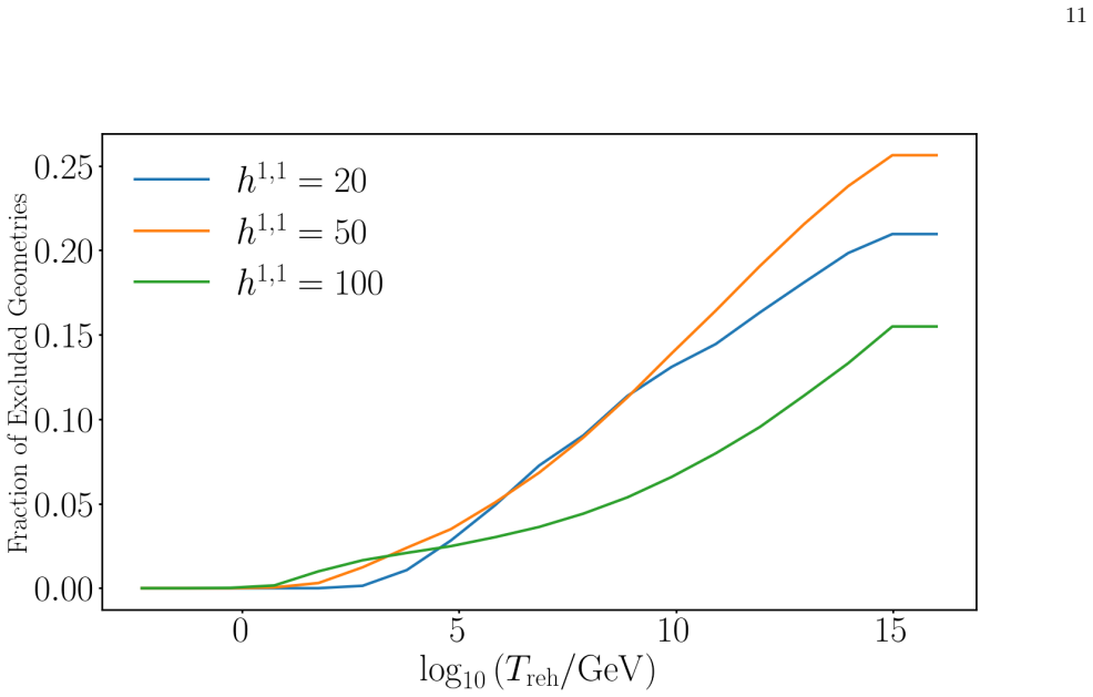
The central claim is that freeze-in production of axions followed by $a\to\gamma\gamma$ decay, tested against the high-redshift component of the CMB optical depth $\tau_{\rm highz} < 0.108$ (95% CL), rules out high reheating temperatures for a definite fraction of explicit string theory models. For $h^{1,1}=20,50,100$, the excluded fractions are approximately 15%, 15%, and 10% at $T_{\rm reh}\gtrsim 10^{10}$ GeV. The calculation follows up to ten axions per model in the mass window $10^5$ eV to $10^{10}$ eV decaying simultaneously, tracks the baryon temperature and ionization fraction with full redshift-dependent energy-deposition efficiencies, and adds a model-independent low-redshift reionization contribution. The paper also produces a single-axion map of the maximum allowed reheating temperature across the $(m_a, g_{a\gamma\gamma})$ plane, which interpolates between low-reheating bounds and the fully thermalized freeze-out regime.
Load-bearing premise
The load-bearing premise is that every sampled Calabi-Yau geometry admits the required orientifold construction even though no such orientifolds are explicitly built; if many geometries fail this test, the ensemble percentages are not percentages of real string-theory vacua.
Editorial extensions
If this is right
- If the central claim is right, about 15% of explicit type IIB axiverse models with $h^{1,1}=20$ or $50$ are incompatible with reheating temperatures above $10^{10}$ GeV, so high-temperature reheating is not automatically safe in string constructions.
- The single-axion map of maximum allowed $T_{\rm reh}$ as a function of $(m_a,g_{a\gamma\gamma})$ provides a direct test for any axion model, including non-string models, once mass and coupling are specified.
- The excluded fraction rises with reheating temperature, reaching roughly 25% at $T_{\rm reh}\approx 10^{16}$ GeV for $h^{1,1}=20,50$, so the tension is strongest exactly in the high-scale reheating regime preferred by many inflationary models.
- Because several axions in one model can decay at different epochs, single-axion limits can miss cumulative injection; the paper's public code computes the full multi-axion history and can be adapted to other decaying relics.
- The same freeze-in-then-decay logic extends to other observables such as X-ray lines, big bang nucleosynthesis, and CMB spectral distortions, but using them will require analogous multi-axion calculations rather than simple single-axion rescaling.
Reading between the lines
- Inference: if the orientifold assumption flagged in the paper fails for a large share of sampled geometries, the reported 15/15/10% fractions should not be read as fractions of actual string vacua; the ensemble would be a sample of polytope triangulations rather than of compactifications.
- Inference: the pipeline is not axion-specific; any dark-matter component produced by freeze-in and decaying to ionizing photons near $z\simeq 20$-$1100$ would contribute to $\tau_{\rm highz}$, so the same public code can be repurposed to test other decaying relics without new formalism.
- Inference: the paper notes that using a better approximation to the Kähler cone strengthens the constraints and becomes more important at large $h^{1,1}$; a more accurate treatment could shift the 10% figure for $h^{1,1}=100$, likely upward.
- Inference: a future CMB polarization measurement that tightens the 95% CL upper limit on $\tau_{\rm highz}$ below 0.108 would sharpen the reheating-temperature boundary and increase the reported model fractions that prefer low $T_{\rm reh}$.
Editorial analysis
A structured set of objections, weighed in public.
Referee Report
Summary. The paper computes the contribution of decaying axions to the high-redshift CMB optical depth in ensembles of explicit type IIB string theory compactifications with h^{1,1}=20, 50, and 100. Axions are produced by freeze-in via the Primakoff process and inverse decay, and their decays are evolved through a full recombination/reionization calculation using DarkHistory deposition efficiencies. The predicted tau_highz is compared with a model-independent 95% posterior upper limit tau_highz < 0.108 from a companion Planck analysis (Paper I). The paper derives, for each model, the maximum reheating temperature consistent with this limit and reports that approximately 15%, 15%, and 10% of models at h^{1,1}=20, 50, and 100 require T_reh <~ 10^10 GeV at 95% CL. A public code for multi-axion reionization is provided.
Significance. If the ensemble construction is accepted, the paper is a significant step in connecting the string axiverse to cosmological data. The multi-axion reionization pipeline with DarkHistory efficiencies is a new tool, and the single-axion maximum-reheating-temperature map (Fig. 8) is a new result in its own right. The freeze-in calculation is cross-checked against the full equilibrium number density (Appendix A, Fig. 12), and the single-axion exclusions reproduce the earlier bounds of Langhoff et al. The central quantitative claim (10-15% of models prefer T_reh < 10^10 GeV) is, however, conditional on an ensemble of toric Calabi-Yau hypersurfaces whose representativeness as type IIB orientifold vacua is assumed rather than demonstrated.
major comments (3)
- [Sec. II.A (footnote 2) and Sec. VI (Fig. 11)] The central result is an ensemble statement: the fractions in Fig. 11 are statistics over the sampled models. But the models are not explicitly constructed as type IIB orientifolds; the paper states 'We simply assume that a compatible orientifold with h^{1,1}=h^{1,1}_+ exists for the given polytope triangulation.' The orientifold projection changes the axion field content, the Kähler metric, and the divisor volumes, and thus can shift the (m_a, g_{aγγ}) distributions that enter the reionization calculation. As the authors note, explicit orientifold construction is now possible in principle (Ref. [48]) and has been implemented at small h^{1,1} (Ref. [31]). The authors should either construct orientifolds for a representative subsample and show that the axion spectra and the resulting fractions are statistically unchanged, or provide a quantitative estimate of the fraction of Batyrev hypersurface triangulations that admit a compatible involution and propagate that uncertainty into the reported fractions. Without this, the abstract's claim of constraining 'explicit type IIB string theory models' overstates what is demonstrated.
- [Sec. VI, Fig. 11] The reported fractions (15%, 15%, 10%) are given without statistical uncertainties. With 500 models per Hodge number (50 polytopes × 10 triangulations), the binomial standard error on a 15% fraction is about 1.6 percentage points, which is comparable to the difference between the h^{1,1}=20/50 results and the h^{1,1}=100 result. The authors should quote uncertainties on the fractions, for example from a beta/binomial posterior, or otherwise justify that the difference between Hodge numbers is significant. This is needed to support the statement that the constraints are weaker at h^{1,1}=100.
- [Sec. VI, text near the mass-window definition] The paper defines a mass window 10^5 eV ≤ m_a ≤ 10^10 eV and selects at most 10 axions per model, stating that 'Empirically, the number of axions within this window rarely exceeds 10 even prior to truncation, so this selection does not bias the physical results.' However, no distribution of the number of axions in the window is shown, and the claim is made for h^{1,1}=50 only (maximum 8). If any model has more than 10 axions in the window, truncation systematically reduces the predicted tau_highz and hence raises the inferred T_MAX_reh. The authors should show the distribution for all three Hodge numbers and quantify the small bias from truncation, or explicitly restrict the ensemble to models with at most 10 axions in the window.
minor comments (6)
- [Abstract and Conclusions] The phrase 'explicit type IIB string theory models' could be softened to 'explicit Calabi-Yau hypersurfaces with an assumed orientifold involution' given the caveat in Sec. II.A.
- [Eq. (7)] The displayed formula for T_fo is difficult to parse; the placement of 'GeV' relative to the parenthesis should be cleaned up.
- [Fig. 3 caption] The Pop-III CCSNe reference line (black) is on a different vertical scale from the axion energy injection curves; the caption should state the units for the black curve.
- [Sec. IV] The definition of tau_highz uses z_c=30 and z_max=800; consider stating explicitly that the standard reionization at z<10 is included only in tau_lowz by construction, which helps interpret the baseline value tau_highz=0.0407.
- [Appendix A] The statement that 'the constraint not to be valid for axion masses significantly above T_reh' is an important caveat; it should appear in the main text near Fig. 6, not only in the appendix.
- [Code availability] The public GitHub repository is a strength; consider providing a versioned DOI or at least a commit hash for reproducibility.
Circularity Check
No circularity: the axion reionization predictions are compared to an externally derived, axion-independent CMB optical-depth limit.
full rationale
The central claim is a comparison between a computed reionization history and an externally derived threshold. The axion parameters (masses and couplings) are not fitted to the tau_highz limit: they come from independently sampled Calabi-Yau geometry via CYTools and the Kreuzer-Skarke database, and T_reh is scanned as a free input. The threshold tau_highz < 0.108 is obtained in companion Paper I [37] from Planck low-ell EE data using a Gaussian-process reconstruction of the ionization history; that analysis does not use axion models, so the comparison is not self-definitional. The freeze-in abundance is computed with fitting formulae from Ref. [39] and checked in Appendix A against the full integral expression, and the single-axion benchmark in Fig. 6 reproduces the independent Langhoff et al. bound. The reliance on Ref. [34] for the ensemble construction is an inheritance of a computational pipeline, not an assumption that the excluded fractions hold; indeed the paper explicitly recomputes the ionization history and improves the Kaehler-cone treatment. The orientifold-existence assumption in Sec. II.A is a stated representativeness caveat about whether the sampled geometries are genuine type IIB vacua; it affects the external validity of the ensemble statistics but does not make any prediction reduce by construction to an input. No equation is shown to be equivalent to another by definition, and no fitted parameter is renamed as a prediction. The self-citations are to independent prior data analyses and code-validated computational tools, not to an unverified premise that decides the outcome. Therefore there is no significant circularity.
Assumptions & free parameters
free parameters (5)
- QCD divisor volume =
40 (string units)
- Electroweak divisor volume bound =
less than 120
- Axion mass window =
10^5 eV to 10^10 eV
- Maximum number of axions per model =
10
- Upper cap on tau_highz =
1
assumptions (7)
- domain assumption Moduli are stabilized with large masses at a point in the stretched Kaehler cone of the Calabi-Yau.
- domain assumption A compatible orientifold with h^{1,1}=h^{1,1}_+ exists for each sampled polytope triangulation.
- domain assumption Axion production from misalignment is set to zero.
- domain assumption Reheating is instantaneous, with no axion production before T_reh.
- domain assumption Energy deposition follows the on-the-spot prescription with redshift-dependent efficiency f_c(z) from DarkHistory.
- ad hoc to paper The union of toric Kaehler cones K_U approximates the true Calabi-Yau Kaehler cone.
- ad hoc to paper The mass window and truncation to 10 axions do not bias the optical depth distribution.
Cite this review
Pith. "Pith review of Constraining the axiverse with reionization." pith.science (2026). https://pith.science/paper/H47NAUW3
@misc{pith2026250703535,
  author       = {Pith},
  title        = {Pith review of: Constraining the axiverse with reionization},
  year         = {2026},
  howpublished = {\url{https://pith.science/paper/H47NAUW3}},
  note         = {Machine review of arXiv:2507.03535}
}
abstract
Axions that couple to electromagnetism are produced in the early Universe by, among other channels, freeze-in via the Primakoff process. For sufficiently large axion masses, the same coupling causes the axions to decay into two photons, which subsequently ionize the intergalactic medium. If this decay occurs in the redshift range $20 \lesssim z \lesssim 1100$, then the contribution to the cosmic microwave background optical depth $\tau_{\rm reio}$ can lead to a conflict with observations, excluding models with sufficiently strongly coupled, heavy axions and high reheating temperatures, $T_{\rm reh}$. Using large ensembles of explicit type IIB string theory models with up to $h^{1,1} = 100$ axions, we compute the full cosmic reionization history caused by the decays of multiple axions. We compare this to the posterior on the high-$z$ component of $\tau_{\rm reio}$ derived from parametric-independent constraints on the ionization state of the Universe, obtained in a full \textit{Planck} analysis presented in a companion paper. For $h^{1,1} = 20, 50, 100$, we find that approximately 15\%, 15\%, and 10\% of the models in the ensemble prefer $T_{\rm reh} \lesssim 10^{10}\,\text{GeV}$ at 95\% CL. We provide a publicly available code at:~\href{https://github.com/ZiwenYin/Reionization-with-multi-axions-decay}{github.com/ZiwenYin/Reionization-with-multi-axions-decay}, which computes the reionization history for arbitrary ensembles of decaying axions. Our analysis opens the door for future large-scale work studying the preference for low-temperature reheating in models with multiple axions.
Figures


Figures from the paper (7 more)



Forward citations
Cited by 5 Pith papers
-
Time-Domain Axion Searches with Magnetic White Dwarfs
The apparent axion-photon conversion signal in PG 1015+014 TESS data is absorbed by the second harmonic of the star's intrinsic light curve, yielding no evidence for axions and a conservative coupling limit.
-
Testing F-theory GUTs with the Axiverse
In F-theory GUTs, non-universal ALPs induced by hypercharge flux satisfy g_aγ/m_a well below the QCD axion prediction when gauge couplings unify near the string scale.
-
Beyond thermal approximations: Precise cosmological bounds on Axion-Like Particles
Solving the momentum-dependent Boltzmann equation and propagating the exact non-thermal ALP spectrum into CMB analyses yields 95% limits f_a>1.63e6 GeV (e), 9.41e6 GeV (mu), 8.06e4 GeV (tau), and g_a_gamma<1.98e-8 GeV^-1.
-
The Atacama Cosmology Telescope: Probing new signatures of ultralight axions with gravitational lensing
New upper limits on ultralight axion dark matter fraction (<1.5% at 10^{-26} eV, <9% at 10^{-25} eV at 95% CL) from combined CMB lensing data, plus marginal 2.1σ preference at 10^{-24.5} eV driven by few points.
-
Axions as Dark Matter, Dark Energy, and Dark Radiation
A mini-review of axion phenomenology showing how light bosons can account for dark matter, drive cosmic acceleration, or contribute to relativistic backgrounds in the early and late Universe.
Reference graph
Works this paper leans on
-
[31]
E. Sheridan, F. Carta, N. Gendler, M. Jain, D. J. E. Marsh, L. McAllister, N. Righi, K. K. Rogers, and A. Schachner, JHEP09, 016 (2025), arXiv:2412.12012 [hep-th]
arXiv 2025
- [48]
-
[1]
R. D. Peccei and H. R. Quinn, Phys. Rev. Lett.38, 1440 (1977)
1977
-
[2]
R. D. Peccei and H. R. Quinn, Phys. Rev. D16, 1791 (1977)
1977
-
[3]
Weinberg, Phys
S. Weinberg, Phys. Rev. Lett.40, 223 (1978)
1978
-
[4]
Wilczek, Phys
F. Wilczek, Phys. Rev. Lett.40, 279 (1978)
1978
-
[5]
L. F. Abbott and P. Sikivie, Phys. Lett. B120, 133 (1983)
1983
-
[6]
Dine and W
M. Dine and W. Fischler, Phys. Lett. B120, 137 (1983)
1983
Show all 73 references
-
[7]
Preskill, M
J. Preskill, M. B. Wise, and F. Wilczek, Phys. Lett. B 120, 127 (1983)
1983
-
[8]
D. J. E. Marsh, Phys. Rept.643, 1 (2016), arXiv:1510.07633 [astro-ph.CO]
2016 arXiv
-
[9]
Di Luzio, M
L. Di Luzio, M. Giannotti, E. Nardi, and L. Visinelli, Phys. Rept.870, 1 (2020), arXiv:2003.01100 [hep-ph]
2020 arXiv
-
[10]
Chadha-Day, J
F. Chadha-Day, J. Ellis, and D. J. E. Marsh, Sci. Adv. 8, abj3618 (2022), arXiv:2105.01406 [hep-ph]
2022 arXiv
-
[11]
C. A. J. O’Hare, PoSCOSMICWISPers, 040 (2024), arXiv:2403.17697 [hep-ph]
2024 arXiv
-
[12]
Masso, F
E. Masso, F. Rota, and G. Zsembinszki, Phys. Rev. D 66, 023004 (2002), arXiv:hep-ph/0203221
2002 arXiv
- [13]
-
[14]
Arias, D
P. Arias, D. Cadamuro, M. Goodsell, J. Jaeckel, J. Re- dondo, and A. Ringwald, JCAP06, 013 (2012), arXiv:1201.5902 [hep-ph]
2012 arXiv
-
[15]
Bolliet, J
B. Bolliet, J. Chluba, and R. Battye, Mon. Not. Roy. Astron. Soc.507, 3148 (2021), arXiv:2012.07292 [astro- ph.CO]
2021 arXiv
-
[16]
Bal´ azset al., JCAP12, 027 (2022), arXiv:2205.13549 [astro-ph.CO]
C. Bal´ azset al., JCAP12, 027 (2022), arXiv:2205.13549 [astro-ph.CO]
2022 arXiv
-
[17]
Langhoff, N
K. Langhoff, N. J. Outmezguine, and N. L. Rodd, Phys. Rev. Lett.129, 241101 (2022), arXiv:2209.06216 [hep- ph]
2022 arXiv
-
[18]
Capozzi, R
F. Capozzi, R. Z. Ferreira, L. Lopez-Honorez, and O. Mena, JCAP06, 060 (2023), arXiv:2303.07426 [astro- ph.CO]
2023 arXiv
-
[19]
H. Liu, W. Qin, G. W. Ridgway, and T. R. Slatyer, Phys. Rev. D108, 043531 (2023), arXiv:2303.07370 [astro- ph.CO]
2023 arXiv
-
[20]
Beaufort, M
C. Beaufort, M. Bastero-Gil, T. Luce, and D. Santos, Phys. Rev. D108, L081302 (2023), arXiv:2303.06968 [hep-ph]
2023 arXiv
-
[21]
F. R. Cand´ on, D. F. G. Fiorillo, G. Lucente, E. Vitagliano, and J. K. Vogel, Phys. Rev. Lett.134, 171004 (2025), arXiv:2412.03660 [hep-ph]
2025 arXiv
-
[22]
Montefalcone, G
G. Montefalcone, G. Elor, K. K. Boddy, and N. Bellomo, Phys. Rev. D112, 023506 (2025), arXiv:2503.00110 [hep- ph]
2025
-
[23]
Witten, Phys
E. Witten, Phys. Lett. B149, 351 (1984)
1984
- [24]
-
[25]
J. P. Conlon, JHEP05, 078 (2006), arXiv:hep- th/0602233
2006
-
[26]
Arvanitaki, S
A. Arvanitaki, S. Dimopoulos, S. Dubovsky, N. Kaloper, and J. March-Russell, Phys. Rev. D81, 123530 (2010), arXiv:0905.4720 [hep-th]
2010 arXiv
-
[27]
B. S. Acharya, K. Bobkov, and P. Kumar, JHEP11, 105 (2010), arXiv:1004.5138 [hep-th]
2010 arXiv
-
[28]
Cicoli, M
M. Cicoli, M. Goodsell, and A. Ringwald, JHEP10, 146 (2012), arXiv:1206.0819 [hep-th]
2012 arXiv
-
[29]
Demirtas, C
M. Demirtas, C. Long, L. McAllister, and M. Stillman, JHEP04, 138 (2020), arXiv:1808.01282 [hep-th]
2020 arXiv
-
[30]
Demirtas, A
M. Demirtas, A. Rios-Tascon, and L. McAllister, (2022), arXiv:2211.03823 [hep-th]
2022 arXiv
-
[32]
V. M. Mehta, M. Demirtas, C. Long, D. J. E. Marsh, L. McAllister, and M. J. Stott, JCAP07, 033 (2021), arXiv:2103.06812 [hep-th]
2021 arXiv
-
[33]
Demirtas, N
M. Demirtas, N. Gendler, C. Long, L. McAllister, and J. Moritz, JHEP06, 092 (2023), arXiv:2112.04503 [hep- th]
2023 arXiv
-
[34]
Gendler, D
N. Gendler, D. J. E. Marsh, L. McAllister, and J. Moritz, JCAP09, 071 (2024), arXiv:2309.13145 [hep-th]
2024 arXiv
-
[35]
Gendler and D
N. Gendler and D. J. E. Marsh, Phys. Rev. Lett.134, 081602 (2025), arXiv:2407.07143 [hep-th]
2025 arXiv
-
[36]
J. N. Benabou, K. Fraser, M. Reig, and B. R. Safdi, Phys. Rev. D112, 066003 (2025), arXiv:2505.15884 [hep- ph]
2025 arXiv
-
[37]
Cheng, Z
H. Cheng, Z. Yin, E. Di Valentino, D. J. E. Marsh, and L. Visinelli, (2025), arXiv:2506.19096 [astro-ph.CO]
2025
-
[38]
Poulin, J
V. Poulin, J. Lesgourgues, and P. D. Serpico, JCAP03, 043 (2017), arXiv:1610.10051 [astro-ph.CO]
2017 arXiv
-
[39]
M. Jain, A. Maggi, W.-Y. Ai, and D. J. E. Marsh, JHEP11, 166 (2024), [Erratum: JHEP 04, 156 (2025)], arXiv:2406.01678 [hep-ph]
2024 arXiv
-
[40]
H. Liu, G. W. Ridgway, and T. R. Slatyer, Phys. Rev. D101, 023530 (2020), arXiv:1904.09296 [astro-ph.CO]
2020 arXiv
-
[41]
Petrossian-Byrne and G
R. Petrossian-Byrne and G. Villadoro, JHEP07, 049 (2025), arXiv:2503.16387 [hep-ph]
2025 arXiv
-
[42]
T. W. Grimm and J. Louis, Nucl. Phys. B699, 387 (2004), arXiv:hep-th/0403067
2004 arXiv
-
[43]
Cicoli, A
M. Cicoli, A. Schachner, and P. Shukla, JHEP04, 003 (2022), arXiv:2109.14624 [hep-th]
2022 arXiv
- [44]
-
[45]
McAllister, J
L. McAllister, J. Moritz, R. Nally, and A. Schachner, Phys. Rev. D111, 086015 (2025), arXiv:2406.13751 [hep- th]
2025 arXiv
-
[46]
V. V. Batyrev, J. Alg. Geom.3, 493 (1994), arXiv:alg- geom/9310003
1994
-
[47]
Kreuzer and H
M. Kreuzer and H. Skarke, Adv. Theor. Math. Phys.4, 1209 (2000), arXiv:hep-th/0002240
2000 arXiv
-
[49]
Cadamuro, S
D. Cadamuro, S. Hannestad, G. Raffelt, and J. Redondo, 13 JCAP02, 003 (2011), arXiv:1011.3694 [hep-ph]
2011 arXiv
-
[50]
L. J. Hall, K. Jedamzik, J. March-Russell, and S. M. West, JHEP03, 080 (2010), arXiv:0911.1120 [hep-ph]
2010 arXiv
-
[51]
P. F. de Salas, M. Lattanzi, G. Mangano, G. Miele, S. Pastor, and O. Pisanti, Phys. Rev. D92, 123534 (2015), arXiv:1511.00672 [astro-ph.CO]
2015 arXiv
-
[52]
Hasegawa, N
T. Hasegawa, N. Hiroshima, K. Kohri, R. S. L. Hansen, T. Tram, and S. Hannestad, JCAP12, 012 (2019), arXiv:1908.10189 [hep-ph]
2019 arXiv
-
[53]
Aghanimet al.(Planck), Astron
N. Aghanimet al.(Planck), Astron. Astrophys.641, A6 (2020), [Erratum: Astron.Astrophys. 652, C4 (2021)], arXiv:1807.06209 [astro-ph.CO]
2020 arXiv
-
[54]
Jaeckel, J
J. Jaeckel, J. Redondo, and A. Ringwald, Phys. Rev. D 89, 103511 (2014), arXiv:1402.7335 [hep-ph]
2014 arXiv
-
[55]
Visinelli and P
L. Visinelli and P. Gondolo, Phys. Rev. D81, 063508 (2010), arXiv:0912.0015 [astro-ph.CO]
2010 arXiv
-
[56]
Escudero, C
M. Escudero, C. K. Pooni, M. Fairbairn, D. Blas, X. Du, and D. J. E. Marsh, Phys. Rev. D109, 043018 (2024), arXiv:2302.10206 [hep-ph]
2024 arXiv
-
[57]
T. R. Slatyer and C.-L. Wu, Phys. Rev. D95, 023010 (2017), arXiv:1610.06933 [astro-ph.CO]
2017 arXiv
-
[58]
Lucca, N
M. Lucca, N. Sch¨ oneberg, D. C. Hooper, J. Lesgourgues, and J. Chluba, JCAP02, 026 (2020), arXiv:1910.04619 [astro-ph.CO]
2020 arXiv
-
[59]
B. D. Fields, K. A. Olive, T.-H. Yeh, and C. Young, JCAP03, 010 (2020), [Erratum: JCAP 11, E02 (2020)], arXiv:1912.01132 [astro-ph.CO]
2020 arXiv
-
[60]
Heinrich and W
C. Heinrich and W. Hu, Phys. Rev. D104, 063505 (2021), arXiv:2104.13998 [astro-ph.CO]
2021 arXiv
-
[61]
Hartwiget al., Astrophys
T. Hartwiget al., Astrophys. J.936, 45 (2022), arXiv:2206.00223 [astro-ph.GA]
2022 arXiv
-
[62]
Aghanimet al.(Planck), Astron
N. Aghanimet al.(Planck), Astron. Astrophys.641, A1 (2020), arXiv:1807.06205 [astro-ph.CO]
2020 arXiv
-
[63]
Domcke and J
V. Domcke and J. Heisig, Phys. Rev. D92, 103515 (2015), arXiv:1504.00345 [astro-ph.CO]
2015 arXiv
-
[64]
Demirtas, L
M. Demirtas, L. McAllister, and A. Rios-Tascon, Fortsch. Phys.68, 2000086 (2020), arXiv:2008.01730 [hep-th]
2020 arXiv
-
[65]
Arias-Arag´ on, F
F. Arias-Arag´ on, F. D’Eramo, R. Z. Ferreira, L. Merlo, and A. Notari, JCAP03, 090 (2021), arXiv:2012.04736 [hep-ph]
2021 arXiv
-
[66]
Caloni, M
L. Caloni, M. Gerbino, M. Lattanzi, and L. Visinelli, JCAP09, 021 (2022), arXiv:2205.01637 [astro-ph.CO]
2022 arXiv
-
[67]
D’Eramo, E
F. D’Eramo, E. Di Valentino, W. Giar` e, F. Hajkarim, A. Melchiorri, O. Mena, F. Renzi, and S. Yun, JCAP 09, 022 (2022), arXiv:2205.07849 [astro-ph.CO]
2022 arXiv
-
[68]
D’Eramo, A
F. D’Eramo, A. Lenoci, and A. Dekker, (2025), arXiv:2506.13864 [hep-ph]
2025
-
[69]
Barbieri, T
N. Barbieri, T. Brinckmann, S. Gariazzo, M. Lattanzi, S. Pastor, and O. Pisanti, (2025), arXiv:2501.01369 [astro-ph.CO]
2025
-
[70]
Halverson, C
J. Halverson, C. Long, and P. Nath, Phys. Rev. D96, 056025 (2017), arXiv:1703.07779 [hep-ph]
2017 arXiv
-
[71]
J. D. Hunter, Computing in Science and Engineering9, 90 (2007)
2007
-
[72]
C. R. Harriset al., Nature (London)585, 357 (2020), arXiv:2006.10256 [cs.MS]
2020 arXiv
-
[73]
Virtanenet al., Nature Methods17, 261 (2020), arXiv:1907.10121 [cs.MS]
P. Virtanenet al., Nature Methods17, 261 (2020), arXiv:1907.10121 [cs.MS]. Appendix A: V alidity of relativistic freeze-in abundance approach A population of axions with massm a, produced by freeze-in from the interaction with a thermal bath at temperature Treh, has number den...
2020 arXiv
Reviewed August 6, 2026 · model on record in the stance chip above.
Discussion (0). Sign in to comment.